A* Optimizations and Improvements

Research Work by Lucho Suaya – Universitat Politècnica de Catalunya

Header

I am Lucho Suaya, a student of the Bahcelor’s Degree in Video Games by UPC at CITM. This content is generated for the second year’s subject Project II, under the supervisión of lecturers Ricard Pillosu and Marc Garrigó.

Index

1. Research Organization
2. Introduction to Problem
   • Before Starting
3. A* First Improvements, Generalities and Context
   • General Improvements and Heuristics Changes
     • Beam Search
     • Bidirectional Search
     • Dynamic Weighting
     • Iterative Deepening (IDA*)
     • Building This Section
   • Paths Recalculations - Incremental Searches
     • Fringe Saving A*
     • Generalized Adaptive A* (GAA*) - Initial Approach to Moving Targets
     • Dynamic A* (DStar) and Lifelong Planning A* (LPA*)
       • LPA* and D*’s son: A love story
   • Angled Pathfinding
     • Field D*
     • Theta*
     • Incremental Phi*
4. Nowadays - Hierarchies and other Games
   • Hierarchical Pathfinding (HPA*)
     • Improving HPA* - Partial Refinement A* (PRA*)
   • Other Games’ Approaches
     • Professor Lupo - Thankful Mention
     • Navigation Meshes and Hierarchy
       • Starcraft II
       • Dragon Age Origins
       • Heroes on the Move
       • Supernauts
     • Hierarchical Pathfinding
       • Castle Story
       • KillZone 2
       • Company of Heroes and Dawn of War 2
5. My Approach - Killing Path Symmetries
   • Jump Point Search (JPS)
     • Introduction
     • Pruning
       • Neighbour Pruning Rules
     • C/C++ Implementation
       • Step by Step Implementation - Do it Yourself Exercise
       • Exercise Solutions
       • Performance
       • More Information on JPS and Sources
   • Other Improvements
     • Rectangular Symmetry Reduction (RSR)
     • Hierarchical Annotated A* (HAA*)
6. Final Thoughts and Recommendations
7. Links to Additional Information
8. Thanks

Research Organization

As you may see in the index, this page has many sections and many information. It’s possible that you are not interested in everything that is explained here, so to ease your accessibility, let me explain how the research is organized (apart of introduction part).

1. First of all, in A* First Improvements, Generalities and Context, I explain the main and minor optimizations for A* and I introduce the concept of Incremental Pathfinding as well as explaining a bit the context in which pathfinding evolved. Finally, I go a bit over angled pathfinding.

2. In the second part, Nowadays - Hierarchies and other Games I start with the Hierarchical Pathfinding approach to improve A*, which is very used and common nowadays, and for that reason, I put many examples of other games using it (in fact, it’s difficult to find big games that do not use it).

3. In the 3rd and final part, I introduce and develop My Approach - Killing Path Symmetries, to improve A * , which is a way to do it developed by an investigator called Daniel Harabor and makes A* way faster. Also, other improvements are explained since JPS might not be the best take for all games, so to have references if it’s your case (although they are not developed as JPS, I put links to works that show how to do it).

Then I conclude this research with final thoughts and some additional information.

You can check a diapositives presentation for this research too (helpful for the later exercise).

Introduction to Problem

As you may deduce, in many games, there is a need to find paths from a location to another, for example, to give a path for a unit to move. To do this, we build algorithms in order to find these paths in an automatic manner. In this research, we will talk about one specific algorithm, which I will suppose you already know, the A*, in order to find optimizations and improvements for it.

A* is a directed algorithm (meaning that it does not blindly search paths) that returns the shortest path between two points (if any). To do it, assesses the best direction to explore, sometimes backtracking to try alternatives. A* is one of the most used algorithms for Pathfinding since it’s pretty fast, so you may ask why do we need to find optimizations or improvements for A* if it already works in a optimal way finding the shortest path existing. The thing is that pathfinding must be performed mostly in real time and with the less resources and CPU usage as possible, specially if there are many objects that need pathfinding (which is much even for A*). Also we need to improve elements such as memory and computational resources, many pathfindings needed at a little amount of time, dynamic worlds, terrain weights, paths recalculations…

So it’s a matter of efficiency; efficiency helps the program running fast and give more importance to other things, so until know, we make it work, and now, we will make it fast, let’s get into it!

Before Starting

Before starting, it’s important for you to know how A* works as well as how grid maps are abstracted in graphs to perform pathfinding and how everything is calculated (if you don’t you can check this page or this one about implementing A*). Also, remember that there are, at least, 3 kind of distance calculations that you can use for heuristics (g values) depending on how do you want pathfinding to work in your game. They are:

• Manhattan Distance for for 4 or 6 directions movement → d = Cl * (abs(dx) + abs(dy))
• Diagonal Movement (8 directions): Chebyshev Distance → d = Cd * max(abs(dx), abs(dy)) for Cd = Cl or Octile Distance for Cd = Cl * sqrt(2) → d = Cl * (dx+dy) + (Cd - 2Cl) * min(dx, dy)
• Euclidean Distance for straight line (any angle/direction) movement, a more expensive calculation and descaling (of g and h) problems → d = Cl * sqrt(2dxdy)

Where Cl is the linear cost (horizontal/vertical) of moving, Cd the diagonal one, dx = x-x0 and dy = y -y0. I’m saying this because you can play with heuristics to change the types of paths you get.

---

*Many information? Looking for other section? Go back to Index

A* First Improvements, Generalities and Context

General Improvements and Heuristics Changes

In this section, I will talk about general A* improvements that can speed up the algorithm. I recommend (if they are used) to mix them with some algorithm explained downwards to a better improvement.

Beam Search

Beam Search sets a limit on the size of OPEN list and, if reached, the elements with less priority are deleted (or which is the same: the elements with less chance of giving a good path). Only the most promising nodes are retained for further branching (reducing memory requirements).

Bidirectional Search

Bidirectional Search is to start two searches in parallel, one from start to goal (being last node found X) and other from goal to start (being last node found Y). When they meet, the search is ended. Instead of doing the A* ’s heuristic, it calculates it as: F = G(start, X) + H (X, Y) + G(Y, goal).

Dynamic Weighting

At the beginning of the search, it’s assumed that is more important to get to the destination rather fast than better, so it changes heuristics to F = G + H * W. This W is a weight associated to the heuristic which goes decreasing as getting closer to the goal, so it goes decreasing the importance of the heuristics and increases the importance of the actual cost of the path, making it faster at the begin and better at the end.

Iterative Deepening (IDA*)

IDA* is an algorithm that can find the shortest path in a weighted graph. It uses A* ’s heuristic to calculate the heuristic of getting to the goal node but, since it’s a depth-first search algorithm, it uses less memory than A*. Even though, it explores the most promising nodes so it does not go to the same depth always (meaning that the time spent is worth). It might explore the same node many times. So, basically, it starts by performing a depth-first search and stops when the heuristics (F = H + G) exceeds a determined value, so if the value is too large, it won’t be considered. This value starts as an estimate initially and it goes increasing at each iteration.

IDA* works for memory constrained problems. While A* keeps a queue of nodes, IDA* do not remember them (excepting the ones in current path), so the memory needed is linear and lower than in A. A good thing of IDA is that doesn’t spend memory on lists since it goes in-depth, but it has some disadvantages that the usage of a base algorithm like Fringe Search can solve (at least partially). This paper explains it deeper.

Building This Section

To build this section, apart of the links used and placed over the text above, I have used fragments of this thesis that explains, among others, interesting things on Heuristics, IDA, A and Fringe Search. Also, I have used a part of this page in Amit’s Thoughts on Pathfinding.

---

Many information? Looking for other section? Go back to Index

Paths Recalculations - Incremental Searches

In this section I will talk about a way to improve and speed up A* through incremental searches which uses information from previous searches to have a basis over which to build the new searches and, therefore, spend less time (speed up searches for sequences of similar problems by using experience from previous problems).

Incremental searches were developed for mobile robots and autonomous vehicle navigation, so it’s a quite deep sector. They tend to have more efficient algorithms than A* (and based on it), but, as they were thought to robotics, they support one only unit in movement, so they might be inefficient for many pathfindings in short times, like the ones we need in games, but it’s good to know them to have a deeper vision on pathfinding.

Fringe Saving A*

Fringe Saving A* launches an A* search and then, if detects a map change, restores the first A* search until the point in which map has changed. Then it begins an A* search from there, instead of doing it from scratch.

Generalized Adaptive A* (GAA*) - Initial Approach to Moving Targets

This variant of A* can handle moving target points. When there is a moving point, the H variable of the heuristics change. If the target is constantly moving, these H values might become inconsistent, so Generalized Adaptive A* (GAA*) updates these H values using information of previous searches and keeps them consistent.

This allows to find shortest paths in state spaces where the action costs can increase over time since consistent h-values remain consistent after action cost increases. It’s easy to implement and understand and better explained in this article.

Dynamic A* (D* ) and Lifelong Planning A* (LPA*)

Dynamic A* (D*) was developed for robotics (mobile robot and autonomous vehicle navigation) to make robots navigate with the shortest path possible and towards a goal in an unknown terrain based on assumptions made (such as no obstacles in the way).

If the robot detects new map informations (for instance, previously unknown obstacles), adds the information to its previous assumptions and, if it’s necessary, it replans a new path. Doing this ensures to have more speed than restarting A* , so D* is for cases in which the complete information is not available, cases in which A* can make mistakes, but D* solves them quickly (making it fit to dynamic obstacles) and allowing fast-replanning. But nevertheless, even though being similar to A*, is more complex and has been obsoleted by a new version which is simpler.

LPA* and D* ’s son: A love story

Parallely, there is an (obsoleted) algorithm called DynamicSWSF-FP that stored the distance from every node to the destination node. It had a big initial setup when calling it, but after graph changes, it updated ONLY the nodes whose distances had changed. This is important for Incremental A* , also called Lifelong Planning A* (LPA* ) which is a combination between DynamicSWSF-FP and A* . In the core, is the same than A* but when the graph changes, the later searches for the same start/finish pairs uses the information of previous searches to reduce the number of nodes to look at, so LPA* is mainly used when the costs of the nodes changes because with A* , the path can be annulled by them (which means that has to be restarted). LPA* can re-use the previous computations to do a new path, which saves time but consumes memory. Although, LPA* has a problem: it finds the best path from the same start to the same finish, but is not very used if the start point is moving or changing (such as units movement), since it works with pairs of the same coordinates. Also, another problem is that both D* and LPA* need lots of space (because, to understand it, you run A* and keep its information) to, if the map changes, decide if adjusting the path fastly. This means that, in a game with many units moving, it’s not practical to use these algorithms because it’s not just the memory used, but the fact that they been designed for robots, which is one only unit moving; if you use them for many units, it stops being better than A*.

So, to fix LPA* ’s heart, it appeared DStar Lite (not based on D* ), mentioned before as it obsoleted D* . Generally, D* and D* Lite have the same behaviour but D* Lite uses LPA* to recalculate map information (LPA* is better on doing so). Also, is simpler to implement and to understand than D* and always runs at least as fast as D*.

---

*Many information? Looking for other section? Go back to Index

Angled Pathfinding

Angled pathfinding is very useful to build more realistic paths and also to improve A* performance. Algorithms allowing this do not only explore from node to node at 45º or 90º like usual, but at any angle thanks to visibility. This means that, instead of just going node per node, if there is a farther node that is visible from the current node (no obstacles in the middle), it will set the parent of the visible node to the current node no matter the angle between both nodes. As said, this makes path to be more realistic while also improving the base A* performance (so we have a win-win!).

For a comparison and explanation between different angled pathfinding algorithms, check out this paper.

Field D*

Field D* is a variant of D* Lite that does not constraints to a grid, it gives the best path moving along any angle adding smooth to the path by using interpolation (which complicates it a bit). It was used for a Mars Rovers, see this paper for more information.

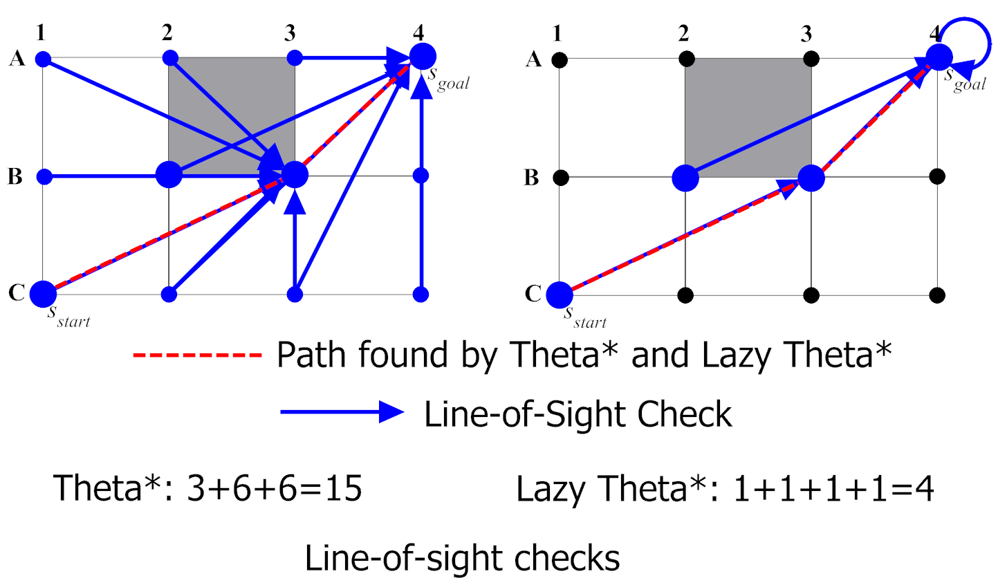
Theta*

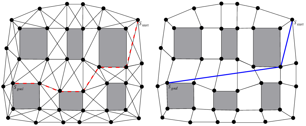
The next is an image of a comparison between A* (in Red) and Lazy Theta* (in Blue, a Theta* improvement):

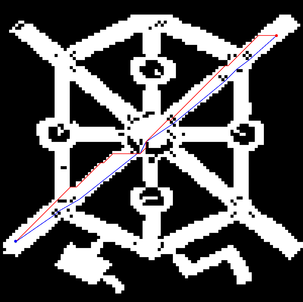
Theta* is an A* and D* variant (like Field D* ) but it doesn’t has fast-replanning capabilities. It runs on square grids and it finds shortest paths that do not strictly follow the grid by pointing to adjacent ancestors, if there is a line of sight towards that node, it can save it as a parent node, skipping the nodes in-between (what is called visibility). See this AI Game Dev article for further information, is well explained there. Also you can see this paper in which there is a longer and deeper explanation on angled pathfinding and also, on Block A*, which is a version of Theta* that is faster because it uses a hierarchical approach (this article gets even more information on Block A*).

Appart of Block A* , there’s also another faster version for Theta* called Lazy Theta* . You can check this AI Game Dev article for more information on it, basically, in four more lines of code, it makes Theta* faster by performing less line of sight checks.

A good advantage of these algorithms is that they are pretty easy to understand and implement.

Incremental Phi*

To finish with angled pathfinding, just mention Incremental Phi* . It mixes Theta* and Field D* , making an incremental version of Theta* (so, allowing fast-replanning). It’s useful for dynamic environments. This paper gets deep into it.

---

*Many information? Looking for other section? Go back to Index

Nowadays - Hierarchies and other Games

On top of the previous researches and especially on top of everything explained in the previous sections, pathfinding started to have different directions. What it seems to be widely used by other reference videogames is the map abstraction into a hierarchy with different levels representing the tiles of the lower levels (that is, dividing the map into areas that, each time with bigger tiles, represent the map itself, like a Quadtree). Before seeing it, let’s see the different types of map representations or how to represent the map in a graph.

Hierarchical Pathfinding (HPA*)

Pathfinding with a large number of units on a large graph, all with different starting locations and potentially different destinations can be tricky and time-performance consuming if there is not a good strategy. Hierarchical pathfinding might solve this problem when needing the previous features. It breaks the graph into a hierarchy and, inside each hierarchy levels, into sectors (called clusters) and performs pathfinding first in the higher levels, and then, in the lower levels that these high-level paths touch. This is that, on a high level layer, a path is planned and then, a second one within clusters of lower level and so. HPA* is used to quickly find an optimal path for many units faster than running A* individually. The number of nodes to check out is lower (since we do smaller searches) and the performance is better.

The hierarchical pathfinding addresses, mainly, three issues (the next parts are very well explained in this AI Game Dev article, which also includes the HPA* paper to download and a evaluation of the algorithm):

1. Dynamic environment and paths changings
2. A* ’s slow performance in big maps
3. Profiting Previous searches (Incremental Search)

And to tackle these, it uses a combination of grid preprocessing to have a high-level graph (with many levels as necessary) using cluster algorithms like Quadtrees, path-planning within the hierarchy (1st at a higher level, then recursively at lower ones) and path re-using.

As you will see, many of the nowadays game uses this approach towards pathfinding. For that reason, you might understand better HPA*, by can check out the next section of this page explaining approaches by other games, especially the ones talking about Castle Story, Heroes on the Move and Killzone.

Improving HPA* - Partial Refinement A* (PRA*)

HPA* also has some improvements. One of them is Partial Refinement A* (PRA* ), that combines the hierarchical map abstraction like HPA* but also connects the different levels of the hierarchy (keeping the current nodes’ connectivity inside a same level), forming kind of pyramids. Then, to find a path, a level of the hierarchy is chosen and search for nodes representing the origin and destination nodes of that path. So, at the higher level chosen, PRA* uses A* to find a path and then projects the first steps down to the next hierarchy levels until reaching the final one (the one in which we need the path to work), where the final path is refined, meaning that is definitively done by considering a corridor around the previous projected path. However, PRA* performance is similar to HPA*.

This paper explains PRA* better and this one purposes an improvement on it.

---

*Many information? Looking for other section? Go back to Index

Other Games’ Approaches

Until here, we have been looking different ways to improve A* ’s performance. Anyway, we should also see how other different games try to overcome the problem to take them as a reference (since they are the ones that have people investigating for their games to work). First of all, to have the first clue, mention that this project is a package for unity that provides an improved A* version and supports different graph set ups (navigation meshes, waypoints…) and even ways to automate them. It’s used by games like Kim, Folk Tale, Divide, CubeMen or Dark Frontier.

I would like to mention that we have tried (with time enough, like a month or two ago) to contact different studios and companies to ask them how they work towards pathfinding, but only two answered. I would like to thank them, one is Beautifun Games (whose we will talk now) and the other is Yatch Club Games, developers of games like Shovel Knight or Cyber Shadow. I won’t talk about them because they answered that they do not use pathfinding in their games since they are simple enough.

In addition, is also helpful to mention that Unity Engine’s Navigation is done with a Miko Mononen’s library that ease all the process of pathfinding and creating Navigation meshes. This library is called Recast.

Without further delay, let’s keep moving!

Professor Lupo - Thankful Mention

Professor Lupo, from Beautifun Games, uses Bresenham algorithm for straight lines. We won’t go deeper into it, but if you are interested, here there is a blog explaining it with code implementation and a check for obstacles blocking the sight between monsters and the player (case in which pathfinding should not be done, and therefore skipping useless calls) and some other features. Red Blob Games has also a page in which explains line drawing with Bresenham and the concept of linear interpolation. Also, you can check a fragment of this book (AI For Game Devs), which explains more deeper the subjects mentioned.

Navigation Meshes and Hierarchy

Starcraft II

The developers of Starcraft II had to lead with hundreds of units moving over a map with different terrains while improving the pathfinding of previous titles (this means, better IA with better and realistic paths). James Anhalt, Lead Software Engineer on Game Systems of Blizzard, explained at GDC 2011 that to attack the problem, they represented the world by using a triangulated Navigation Mesh** over which A* is run. As they needed to save a lot of memory, and to make it more faster, they statically allocated everything and condensed the structures into 16 bytes per face of triangle and 4 bytes per vertex, which allowed to have 64000 faces and 32000 vertices.

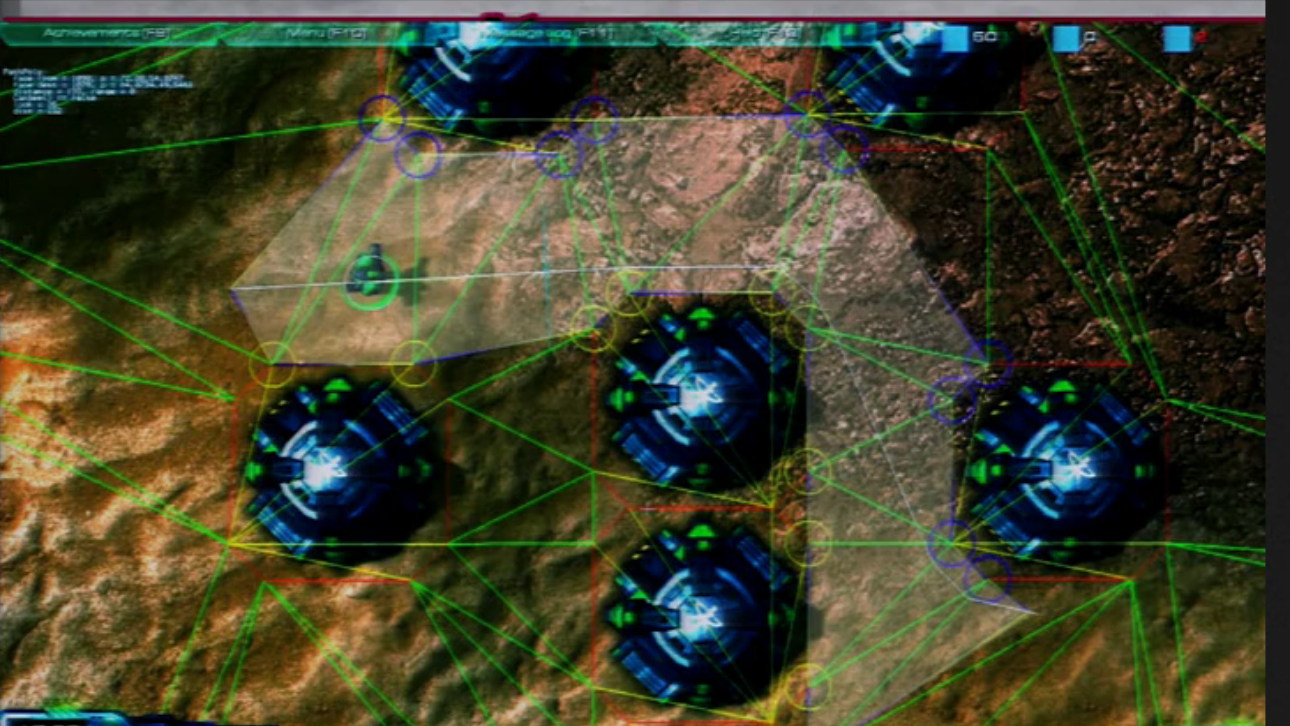
I won’t talk more about Starcraft II pathfinding since it’s not in the direction of this research, but if you want to know more, you can go to that 2011 GDC talk in which he explains it deeper (minutes 3 to 20), which is the same talk in which the orators explain the pathfinding for Heroes on the Move and Dragon Age Origin. Also, check the section 2.4 (Triangulation Based Pathfinding) of this Pathfinding book (pages 24-25) that explains a bit about Pathfinding with triangulated map representations.

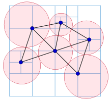
Specifically, Constrained Delaunay Triangulation, which is a generalization of the Delaunay Triangulation that not always accomplishes a rule called the Delaunay Condition that states that the circle circumscribed of each triangle dividing, in this case the map, cannot contain any vertex of other triangle. A Triangulation is the division of the map into triangles, for the people who does not know.

Probably they used this to build a Navigation Map in which use a pathfinding algorithm on top.

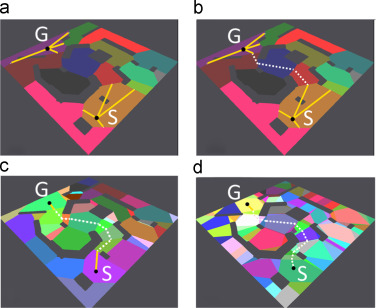
Dragon Age Origins

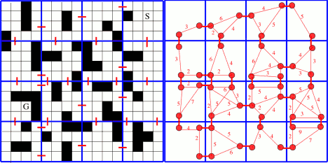
The case of Dragon Age Origins is similar to the ones of its same talk in GDC 2011 talk (minute 36 to 54), Starcraft II and Heroes on the Move, and as they were before, Nathan Sturtevant (consultant for BioWare that implemented pathfinding engine) do not explain a lot regarding to pathfinding itself since it seems pretty similar to the previous talks, so it focuses more on path smoothing, quality and trap avoidance (how to prevent pathfinding to make weird things and make it look good). As told, Dragon Age’s approach is similar to the previous: they hierarchize the map in a low level graph (represented by grids) and a higher level to make the world movement (represented by a kind of a Navigation Mesh). Also, they divide the whole map in sectors and sub-sectors (called regions). Their goals towards pathfinding were to achieve a fast planner while planning long paths and being memory efficient. The next are images of a prototype for Dragon Age with a low level grid representation (red) and the second image has, in yellow, the representation of the high level grid.

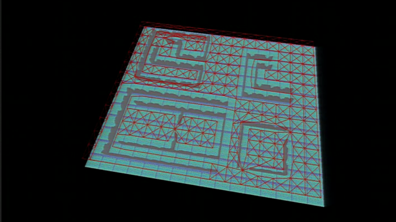
Just for curiosity, he mentions that they use octile heuristics. Also (and because of curiosity too) it mentions that Google can perform fast pathfinding because they rely a lot on roads properties (highways are the faster way to get somewhere).

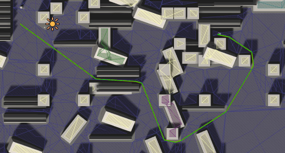
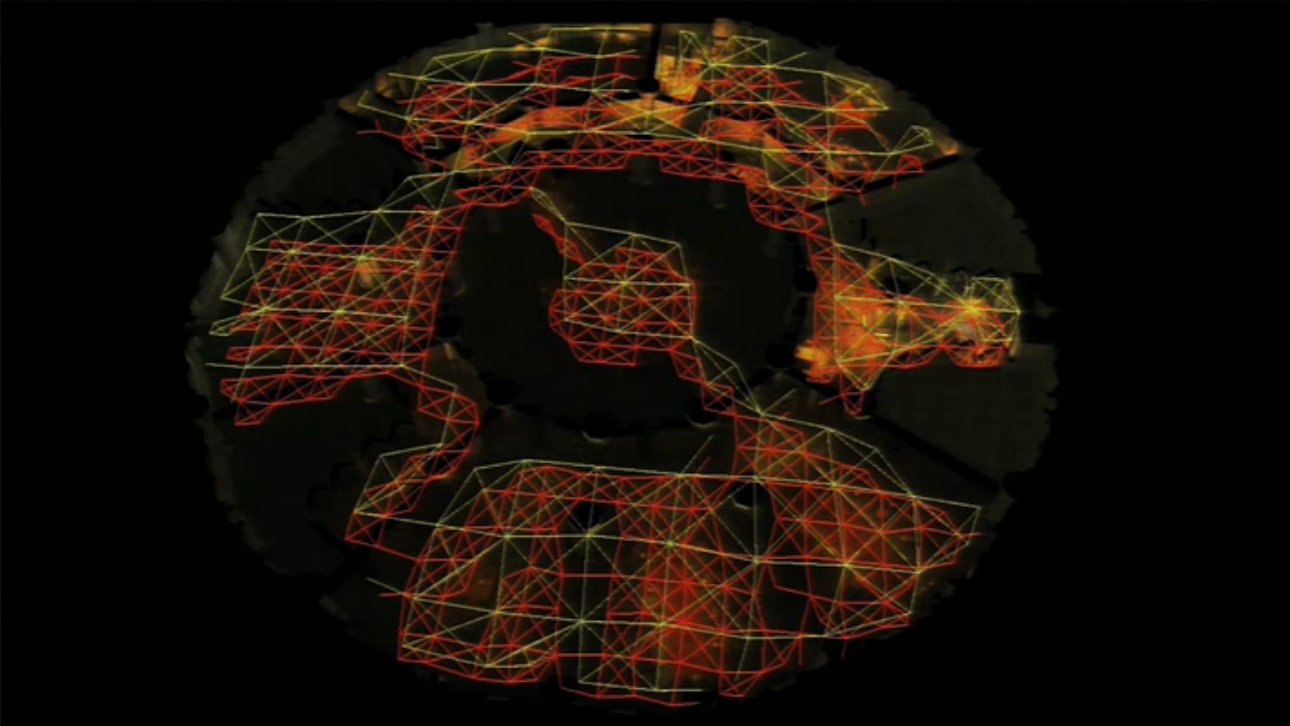
Heroes on the Move

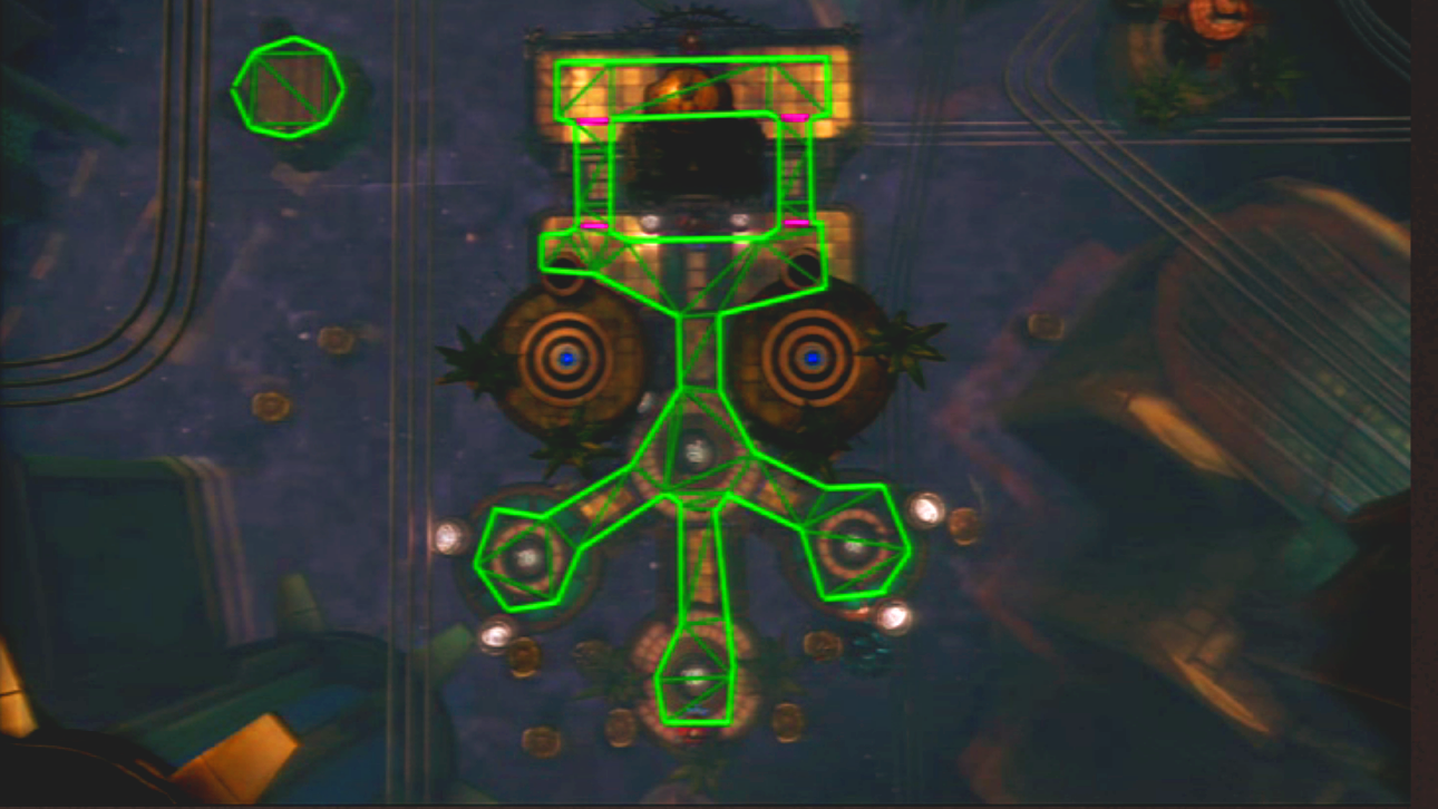
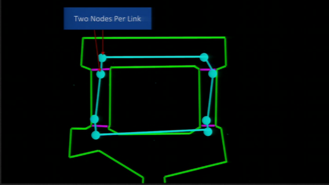
The Playstation’s Heroes on the Move developers had to come up with a solution that allowed runtime planning of pathfinding while spending no more than the 50% of the time on navigation, so they did something similar to Starcraft II but they also applied hierarchy levels and calculate paths in them to smooth them later. First of all, they triangulated a Navigation Mesh.

With this, they have a high level (with two nodes per cell):

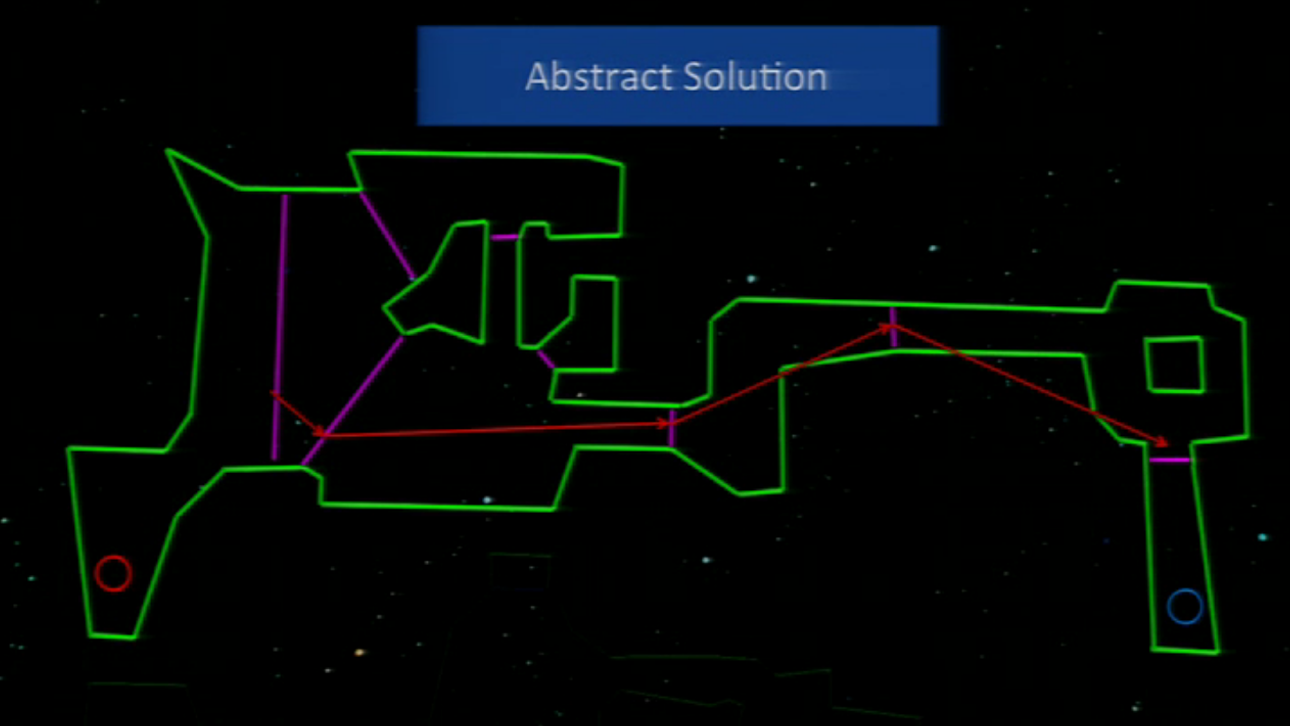
And, when they wanted to find a path, they found a solution first in the abstract graph:

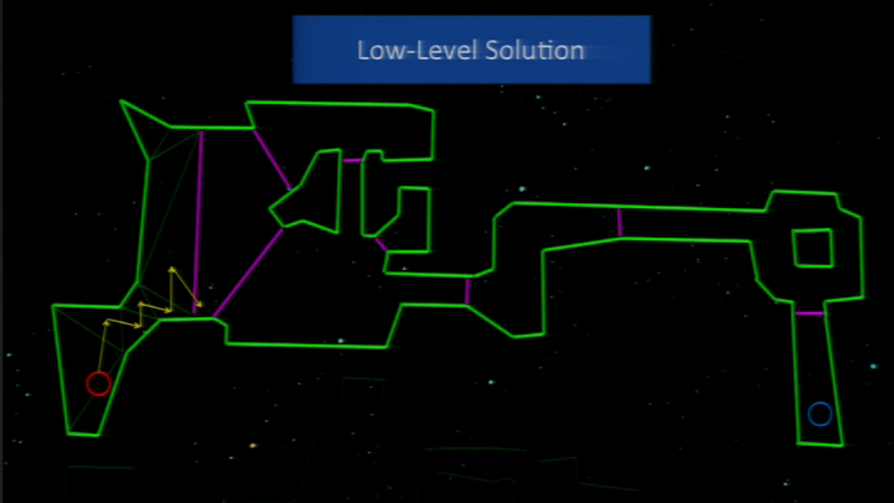
And then they went, in the abstract graph, area per area building a path. This means that, once they have an abstract solution, first pick an area and do the path inside and then the other and so while the game keeps running. Like this:

And when the element moving arrives to the “portal” (the frontier between areas), they calculate the path to the next area. This allows what they seek: to pathfind in runtime and keeping it fast (not spending much time). To know the place where to cross between lines, they just calculated the nearest point to the moving element.

This pathfinding way is also explained in the same GDC 2011 talk than Starcraft II and Dragon Age Origin (from minute 20 to 36).

Supernauts

Harri Hatinen, Lead Programmer of Grand Cru, explained in the GDC China 2014 that they abstracted the map to a Navigation Mesh and mixed with hierarchy representation for Supernauts. I could recover the presentation in which explains how they handle the navigation map, how they make it work (taking into account the frontier between nodes and its longitude, How the IA knows where to pass by in a large frontier between nodes?) and how they update it each time that the map changes.

There is a video of that presentation, but it’s a little annoying to hear a chinese voice over the Harri Hatinen’s viking’s voice (and the video quality is a bit low, but with the diapositives it can be understood).

Hierarchical Pathfinding

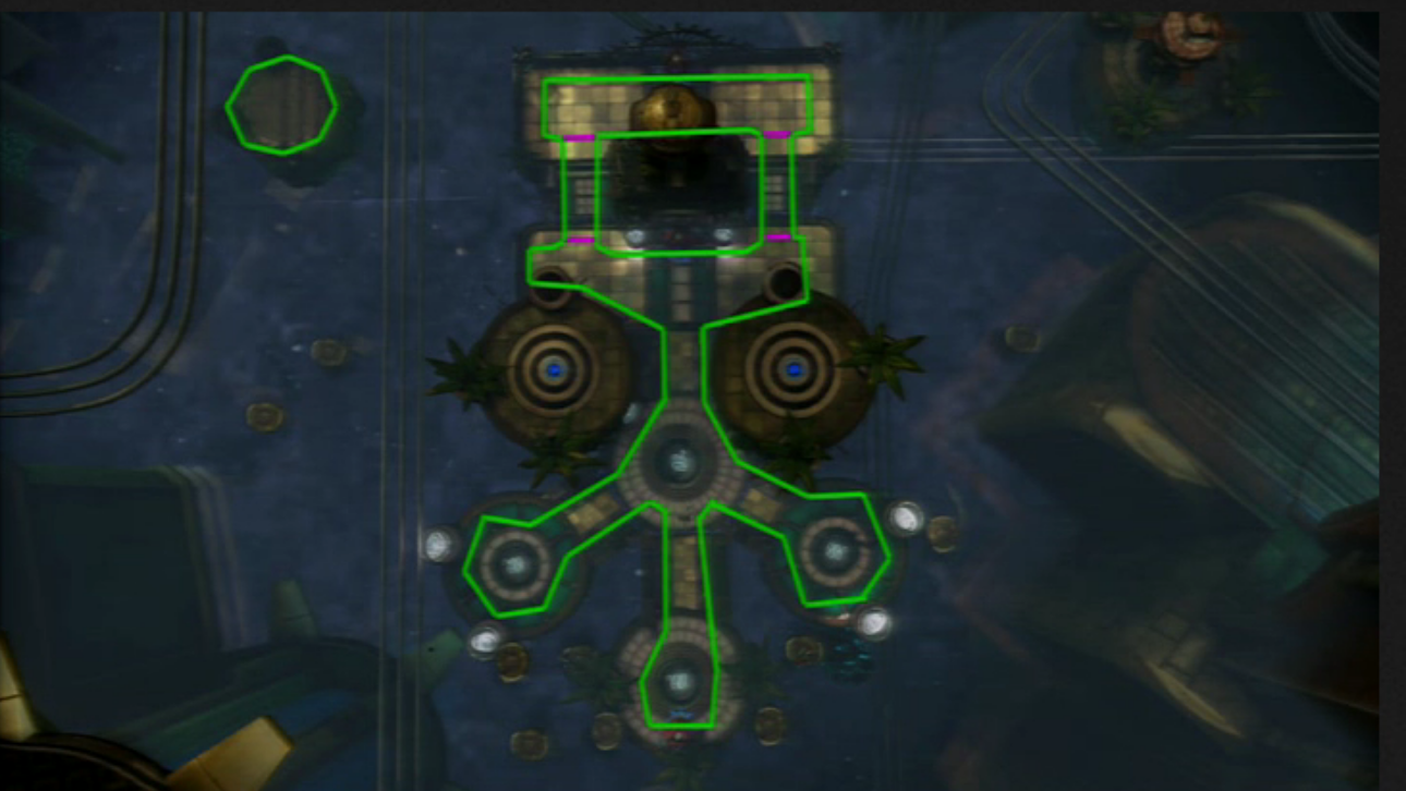
Castle Story

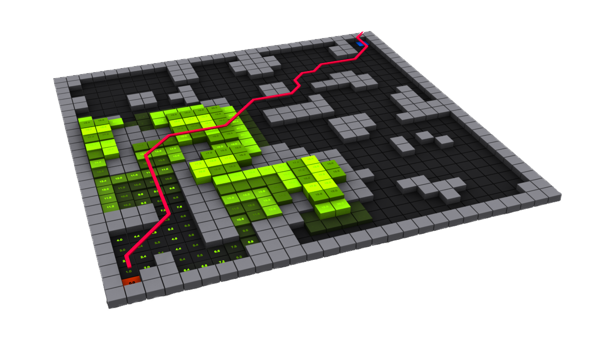
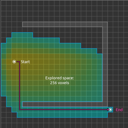
Another interesting talk, this case in the GDC 2018, was the one by Alain Benoit, Lead Programmer and CTO (Chief Technology Officer) of Sauropod Studio. I could only find the diapositives’ presentation because to see the video you must be a GDC member (which I’m not, I’m a student and sadly I don’t have 550$ each year to invest in GDC), but in case you are, I leave you the search of that presentation here. Anyway, with the diapositives it’s pretty understandable that for their game, Castle Story, they decided to use Hierarchical Pathfinding to fulfill their needs to have many agents moving, dynamic obstacles, stairs and blockages, deformable terrain and buildable blocks in a large scale map.

Note that they mention all this for Voxel worlds (worlds built from cubes called Voxels instead of triangles, as traditionally), and I’m not sure how this can affect the research or the pathfinding; probably the map abstraction is a bit different.

The truth is that this way of solving pathfinding problems is very effective and it solves them in a fast way. So, as told, they us hierarchy to abstract the grid and improve pathfinding efficiency, see it with images:

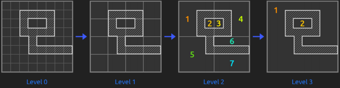
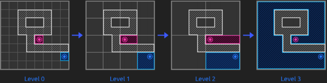
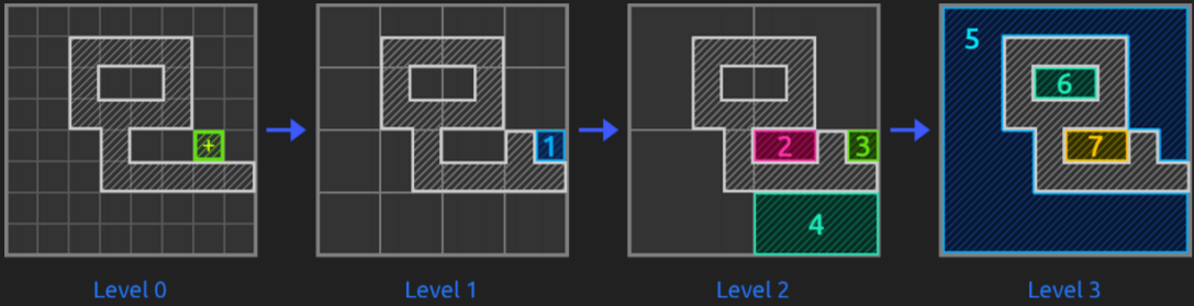
To find optimum paths, they state a certain chain of rules such as explore lower hierarchy levels as getting closer to the goal, or exploring them if they have dynamic obstacles, not exploring childs if parents already were…

KillZone 2

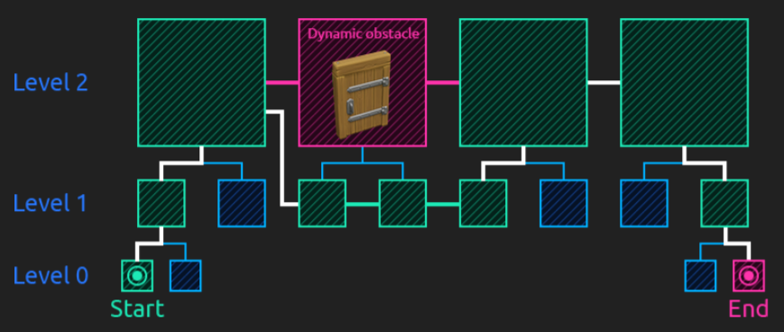
I can’t talk that much about Killzone 2 since the only thing I have is this power point from the Game AI Conference celebrated in Paris in 2009. From the diapositives I could translate and extract that they use kind of a mix between waypoints and hierarchy (a set of areas created as groups of waypoints):

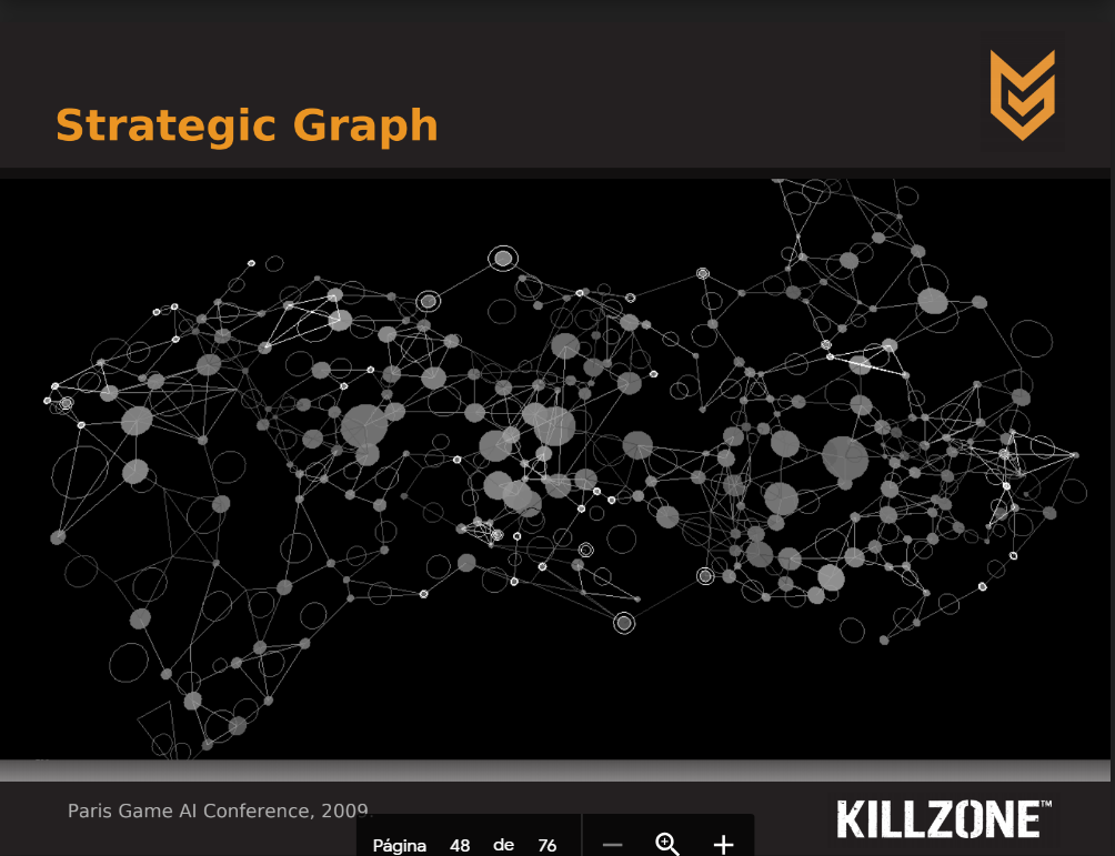
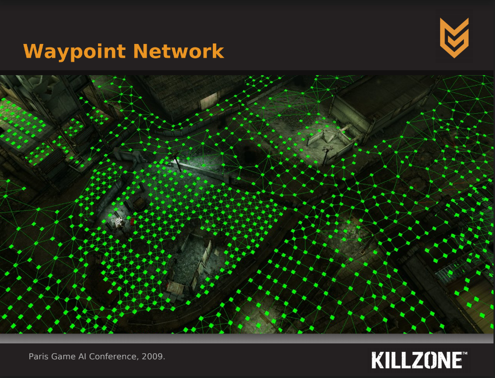
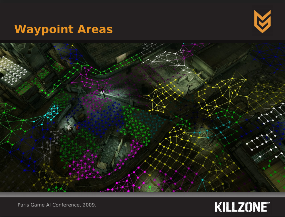
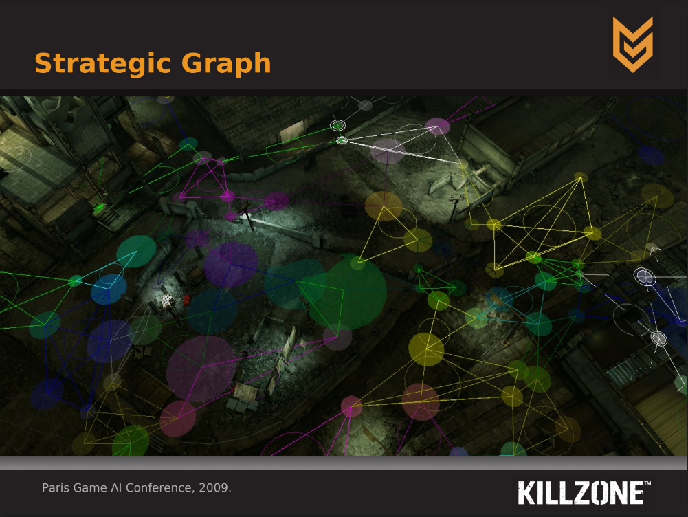
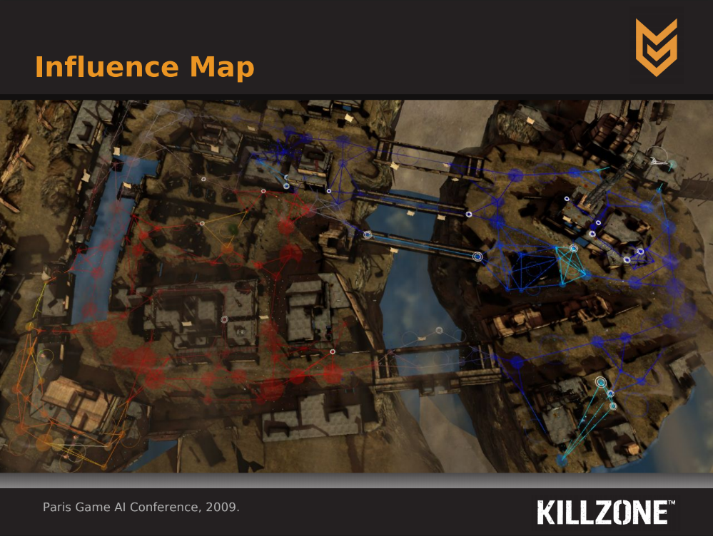
This is for supporting strategic decision making algorithms. They do a high-level graph based on the low-level waypoint network and use an automatic area generation algorithm. So, they have dynamic information over the strategic graph for many decisions (hide, defend, regroup…) and to store some influence information based on faction controls of the area, and they calculate it based on all bots, turrets… They put an example of this.

Over this, they work with pathfinding. Think that the game needs to make strategic decisions taking into account the previous strategic and influence graphs. So, they use a single-source pathfinder to calculate distances to a point, the algorithm combines Dijkstra and Bellman-Ford-Moore (paths from a single-source from all other vertices in a weighted directed graph, slower than Dijkstra but more versatile since handles nodes with negative numbers), but with some tricks to make it more efficient and improving the distance estimates (the heuristics) when multiple updates. Now from here, each squad of units has an own pathfinder which finds a path between waypoints in the selected areas.

Again, this is a translation with some interpretations of the powerpoint linked above, I’m not 100% sure on how it actually works since I can’t go deeply on it with only this presentation, so I might be wrong in something.

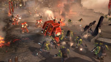
Company of Heroes and Dawn of War 2

The AI Game Dev platform (sadly seems closed by now, check the page in the past from the internet web archive, was a really nice page about AI), interviewed Chris Jurney, which worked as Senior Programmer in Relic Entertainment and at Kaos Studios. It was part of the development of Company of Heroes and Dawn of War 2, games for which he was interviewed in the interview that I’m talking about. You can see the transcription in PDF and the MP3 recording.

In there, he explains that the pathfinding in Company of Heroes worked as well with Hierarchical Pathfinding in a map of thousand of meters (so thousands of cells) in which the worst case was 1000x250 (250 000 cells). This was very complicated to implement (especially for map changes and updates), so he says that HPA* can be a good complexity-decrementer (event thought it confesses that he did not tried).

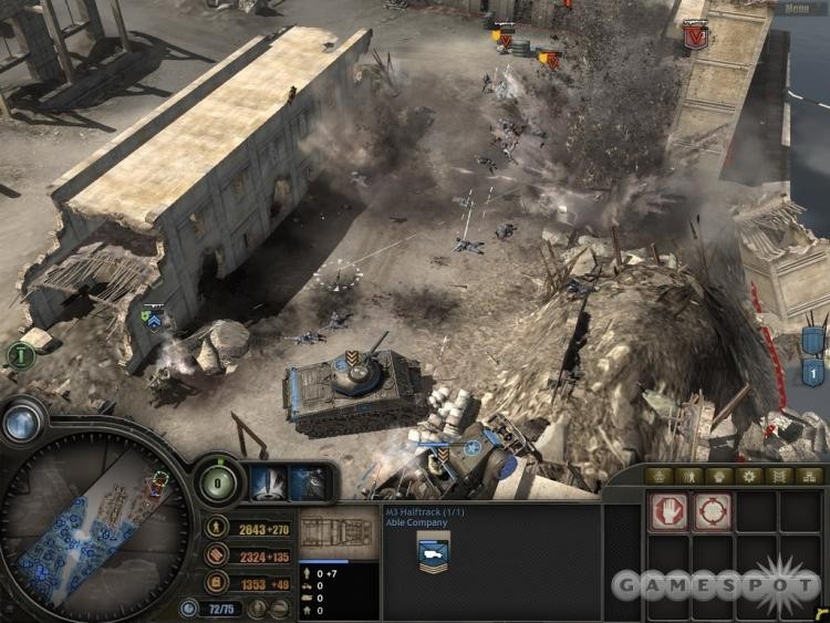
With hierarchical pathfinding, he says that each unit can recalculate behaviour each 3/10 to half a second to follow a leader that actually knows the whole picture and re-evaluates the route every second. In the GDC China 2007, this man, along with Shelby Hubick give a presentation about AI in Destructive environments in Company of Heroes, in case you are interested in it. This is the Audio (again, couldn’t find a video, sorry). In fact, I recently discovered that in this article of AI Game Dev about Clearance Pathfanding and HAA* , is said that Chris Jurney, in that GDC 2007 talk, explains that they use a similar method to HAA* (explained downwards) with the usage of a variant of Brushfire algorithm to put numeric values to the tiles of the map according their nearness to an obstacle and, therefore, calculating if the size of a troop make it able to pass through an area. The reason why this is not very well explained here is because is not completely shared in the talk and the article about it in the AI Game Dev page is premium (and I cannot have access). Anyway, you have a similar approach detailed downwards if you are interested (HAA* section).

---

*Many information? Looking for other section? Go back to Index

My Approach - Killing Path Symmetries

In this section I will explain my approach to improve as much as possible the A* pathfinding taking into account the projects of video games creation that we are developing for a University’s subject, in which we will need a pathfinding fast as possible, but it might serve for any reader or other projects, too. I will deeply explain Jump Point Search algorithm because is the one that best fits into my team’s project, but I will also leave an explanation of two other systems called Rectangular Symmetry Reduction and Hierarchical Annotated Pathfinding, just in case that Jump Point Search does not fit to your requirements. Anyway, I won’t explain deeply its development (unlikely JPS) because of space and time matters, but I will let you some documentation so you can access to the information needed to implement it in case you need it.

Before going into it, let me explain what a path symmetry is. As you may guess, from a starting point, there might be many ways to reach a destination, this means that for the same start/destination, there can be many paths. Well, symmetric paths are these kind of paths in which the only difference is the places they pass by. The formal definition is: “Two paths in a grid are symmetric if they share the same start and end point and one can be derives from the other by swapping the order of the constituent vectors”. They would look like:

A* explores all the paths even if they are symmetric, so it makes lots of useless efforts and searches traduced in decreasing performance, so many approaches to improve A* focus on killing or avoiding path symmetries, having great results. In this page, we will see two of them, but we will focus especially on one, explaining its development, an algorithm A*-based called Jump Point Search. This page contains more information about this (but I think it was clearly explained and does not needs further expanding, I place the link here to make you know that the information comes from there).

Jump Point Search (JPS)

Introduction

Jump Point Search is a grid-specific algorithm developed by Daniel Harabor and Alban Grastien in 2012 under the supervision of the NICTA (Papua New Guinea Information and Communications Authority) and the Australian National University. The algorithm expands by choosing (pruning) certain nodes in the grid map (called Jump Points) while the intermediate nodes are not expanded (skipping the exploration of a lot of nodes). The technique used by JPS, is based on avoiding useless searches of symmetrical paths that A* do, saving lots of time with the same memory load.

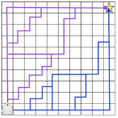
In the article in which they present it, they prove that JPS computes always optimal solutions and is way faster than A* (over an order of magnitude, meaning that can be until a thousand times faster, as shown in this video). Also, it does not have memory overloads, in contrary of Hierarchical Pathfinding, which gives, although fast, sub-optimal paths (more useful than better solutions) while having small memory overloads. In the above picture’s case, the node x (with parent p(x)) in the standard A* version, would open up all the traversable neighbours around, but JPS would just go to the right and keep moving towards that direction until finding a node such as y (a Jump Point) and then generate it as successor of x and assigning it a G value. In case that y was an obstacle, JPS assumes that it has to stop searching towards that direction.

Pruning

Moving from a Jump Point to another is done by travelling in a concrete direction while recursively applying two neighbour pruning rules (one for horizontal and vertical steps and the other for diagonal ones) until reaching a dead-end, a non-walkable area or the next Jump Point. To keep going on with JPS, is important to understand the concept of “pruning”, which is the elimination of nodes to expand. This is to say that is the way in which the algorithm decides which nodes to explore. Take into account that the definition of pruning is “to trime (a tree, bush…) by cutting away dead or overgrown branches or stems, especially to encourage growth”. Actually, nodes are trees in the eyes of pathfinding algorithms, so it actually make sense the use of the word.

After the pruning of nodes, the ones that remain in the tree are called “natural neighbours” which are the only ones that we want to consider. However, sometimes we will need to consider one or two nodes (because obstacles or something) that are not natural itself. Those are called “forced neighbours”.

Now, we are ready to get to work with Jump Point Search!

Neighbour Pruning Rules

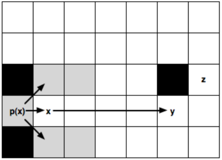
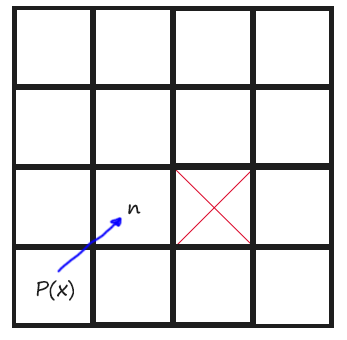
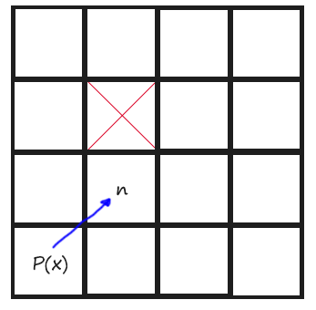
In Jump Point Search, our objective will be to avoid symmetric paths by “jumping” all nodes that can be optimally reached by a path that does not visit the current node (thanks recursive magic!). This means that we chose a Jump Point if the optimal path must, obligatory, pass through that node. Once it has reached an obstacle or another Jump Point, the recursion stops. So a Jump Point y with a neighbour z will be a successor of a Jump Point x only if to reach z we need to visit x and y. To make it real, we need to consider two pruning rules, one for straight moves (horizontal and vertical) and another one for diagonal moves.

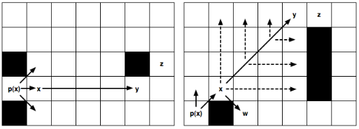
In the left image, from a Jump Point x (with parent p(x)), we recursively go straight until y and set it as a successor Jump Point of x because z can’t be reached (optimally) if we don’t pass through x and y. The nodes in the middle are not evaluated or explored. In the right image, from a Jump Point x (with parent p(x)), we recursively go diagonally until y and set it as an x Jump Point Successor (the same than left). In this case, after each diagonal step, we do a recursion straightly (marked with discontinue lines) and only if the two straight recursions fail, we keep going diagonally. Also in the image, the node w is shown, which is a forced neighbour of x because of being in a place in which, to reach it optimally from the coming direction (p(x)), we need to pass through x.

C/C++ Implementation

In this part, we will see how to properly implement Jump Point Search in C/C++. In order to do that, we will do an exercise step-by-step to learn how to build it, and then I will put the solution for that exercise. You can download both the exercise and the solution here, in my research repository of GitHub. If you do, have into account that is a modular system (take into account only the Scene Module, which is the one that asks for paths and the Pathfinding Module, the one actually doing them). First of all, let’s see what’s new from A*. We have three new functions:

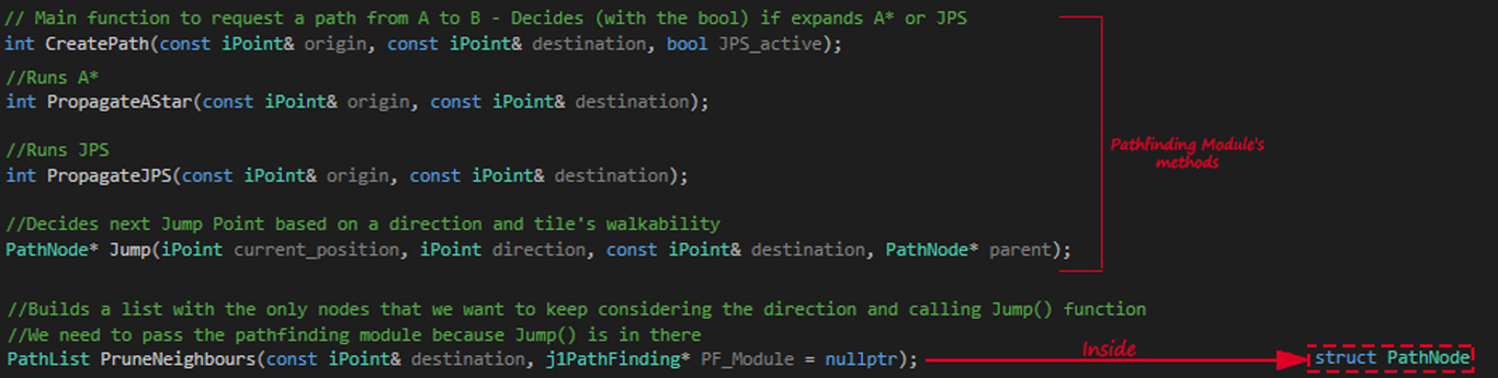
• PropagateJPS() - Runs the algorithm. Is kept equal to PropagateAStar() but with the exception of a line deciding each tile’s neighbours.
• Jump() - Decides, recursively, which will be the next Jump Point from the current node based on direction and walkability
• PruneNeighbours() - This one is inside each PathNode structure (meaning that only can be called through a tile of PathNode type).

The other functions in the image are the PropagateAStar(), which is self-explanatory, and CreatePath(), that is called each time we want to compute a path and decides, based on the bool that is passed, if calling JPS or A*. So, now that we have seen what’s new (is not much, right?), we can start with the exercise!

Step by Step Implementation - Do it Yourself Exercise

Our goal now is to go step by step implementing JPS in order to understand how it works and how to build it. Before starting, it would be good if you just go around the pathfinding module seeing and trying to understand, conceptually, what the functions explained in the previous explanation do. So, if you download the exercise linked again here, the exercise folder is the one called “Handout”. In there, there is the code with the exercises to do, but also a folder with an executable showing how the result should look like (inside Game folder). You can play with it a bit to check the A* and JPS visual and performatic differences. Then, if you go to the exercises code, you will see that nothing happens if you call JPS (if you call A*, this one is already done to do the path). So let’s begin.

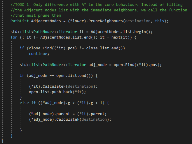
Todo 1

After checking the header for pathfinding module, we must go to the JPS core, the PropagateJPS() function. In here, there is one only difference with the PropagateAStar() function, which is how the current node’s neighbours are filled. In A*, we called the FillAdjacents() function to fill a list with the immediate neighbours, but now, in JPS, we must prune them.

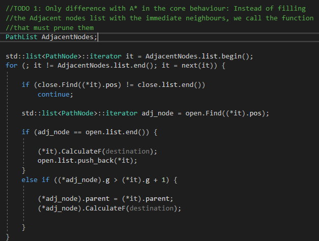
You won’t see anything of JPS working until TODO 4 (but to find a path with the same start/goal node because of its core that calls him). The ms showing can change because they measure the time that lasts calling the PropagateJPF() function and, of course, A* because is already done and you don’t need to do it (it’s not the exercise focus), take it into account.

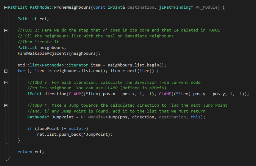
Todo 2

Now let’s go to the PruneNeighbours() functions in which we will do the incoming TODOs. First, in TODO 2, we must create and fill a list with the immediate neighbours of the current node (just as A* do, the step that we deleted in JPS core). Then iterate that list.

Next is an image of TODOs 2, 3 and 4:

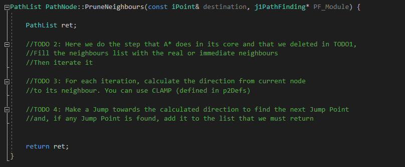
Todo 3

Once the second TODO is done, inside each iteration, we must calculate the direction from the current node to its neighbour that is currently being iterated. Remember to use CLAMP method, defined in p2Defs header (inside Core/Tools) to keep the direction inside a unitary factor (between -1 and 1).

On the next Todos, JPS will start working, until now you shouldn’t have been able to see nothing from JPS.

Todo 4

Once the direction is calculated, perform a Jump towards that direction to find the next Jump Point. Then, if any one is found, add it to the list that we must return (already created).

If this is done correctly, JPS should be able to find strictly straigh paths (or horizontals or verticals but not mixes or with colliders in the middle) that will show only the goal and start nodes as this:

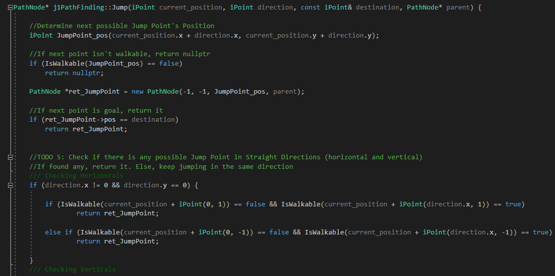
Todo 5

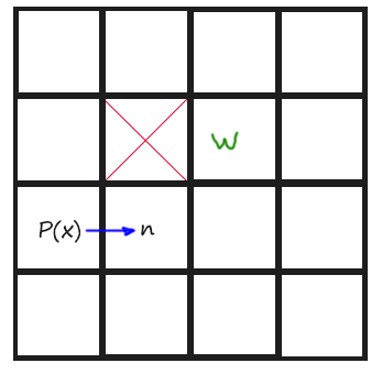
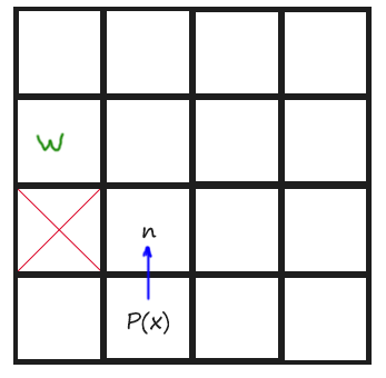
Now is time to code the Jump() function. Let’s begin by determining how the algorithm, according to the rules stated, must explore towards straight directions (horizonals and verticals). Remember that we just have to keep looking until finding a Jump Point. To remember those rules and give them a more coding meaning, if we are coming horizontal, a Jump Point is found when one of the tiles aside the current position in Y axis is not walkable and the one at +X direction of that non-walkable tile, is walkable. And if we are coming vertically, a Jump Point is found when one of the tiles aside the current position in X axis is not walkable and the one at +Y direction of that non-walkable tile, is walkable. You might understand it better with a drawing:

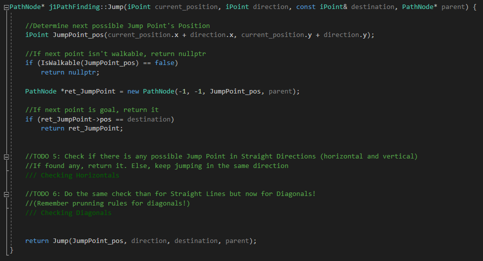
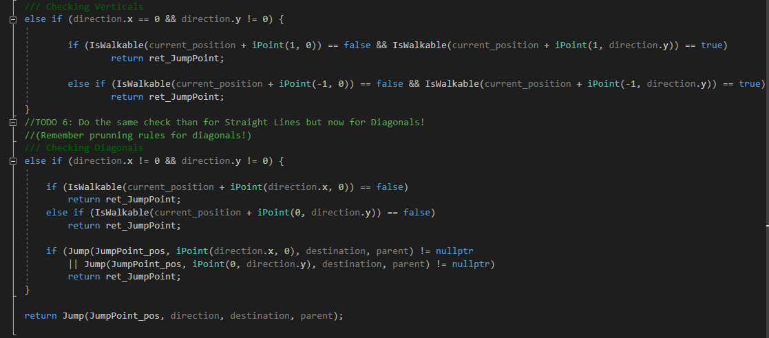
Next is an image of Todos 5 and 6:

If some Jump Point is found, return it. Otherwise, just keep exploring with recursive magic. By now, you should be able to build (only) straight paths JPS (as in TODO 4 but with the nodes explored in the middle) and see their speed difference (and the steps taken by each one in output console of Visual Studio):

If you change the heuristics in the function CalculateF() and select the DiagonalDistance() to calculate H values, you can build some paths with JPS that are not only straight in itself, but all its parts are formed by straight paths (with colliders in the middle), like this:

Todo 6

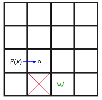
Finally we have to do the same than TODO 5 but with diagonal directions. Diagonal directions had other rules. To give them a more coding definition, a Jump Point is found diagonally when the tile aside the current position in X direction or in Y direction is not walkable. I have made a drawing for this too:

Also, if, from the current point, there is no possibility on Jumping towards X direction or towards Y direction, then we have also found a Jump Point.

In the function FindWalkableAdjacent(), remember to uncomment the lines that fill the list with diagonal tiles to be able to go diagonally.

Now the whole exercise is totally done. The result should look like in the solution executable in Game folder. You should be able to build any path with both algorithms and see the efficiency differences (and steps taken by each one in output console of Visual Studio).

Exercise Solutions

Now I will show you the solutions for the previous TODOs to complete the exercise and have the resulting JPS. I think they don0t need further explanations.

Todo 1

Todo 2, 3 and 4

Todo 5

Todo 6

Performance

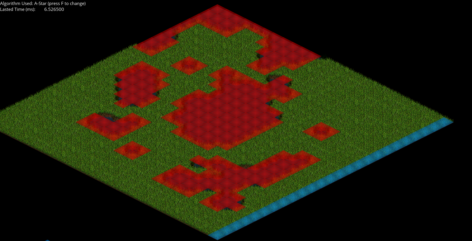
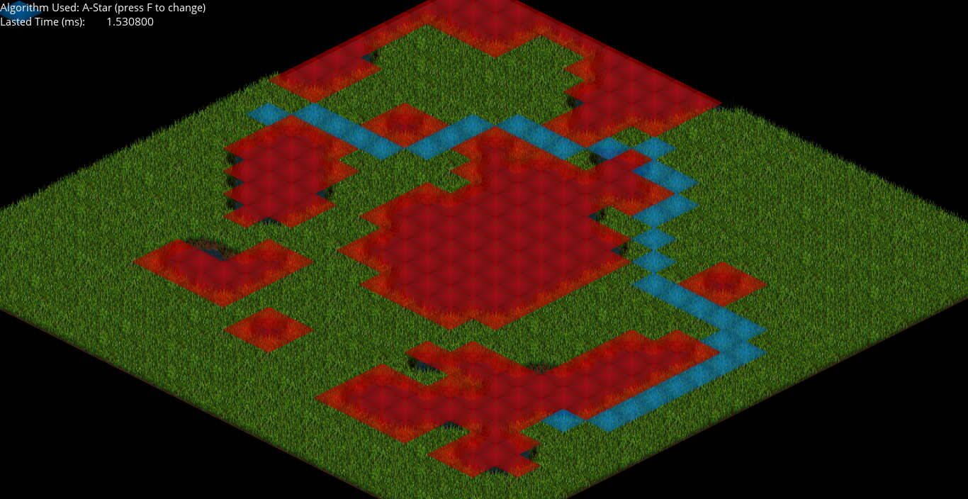
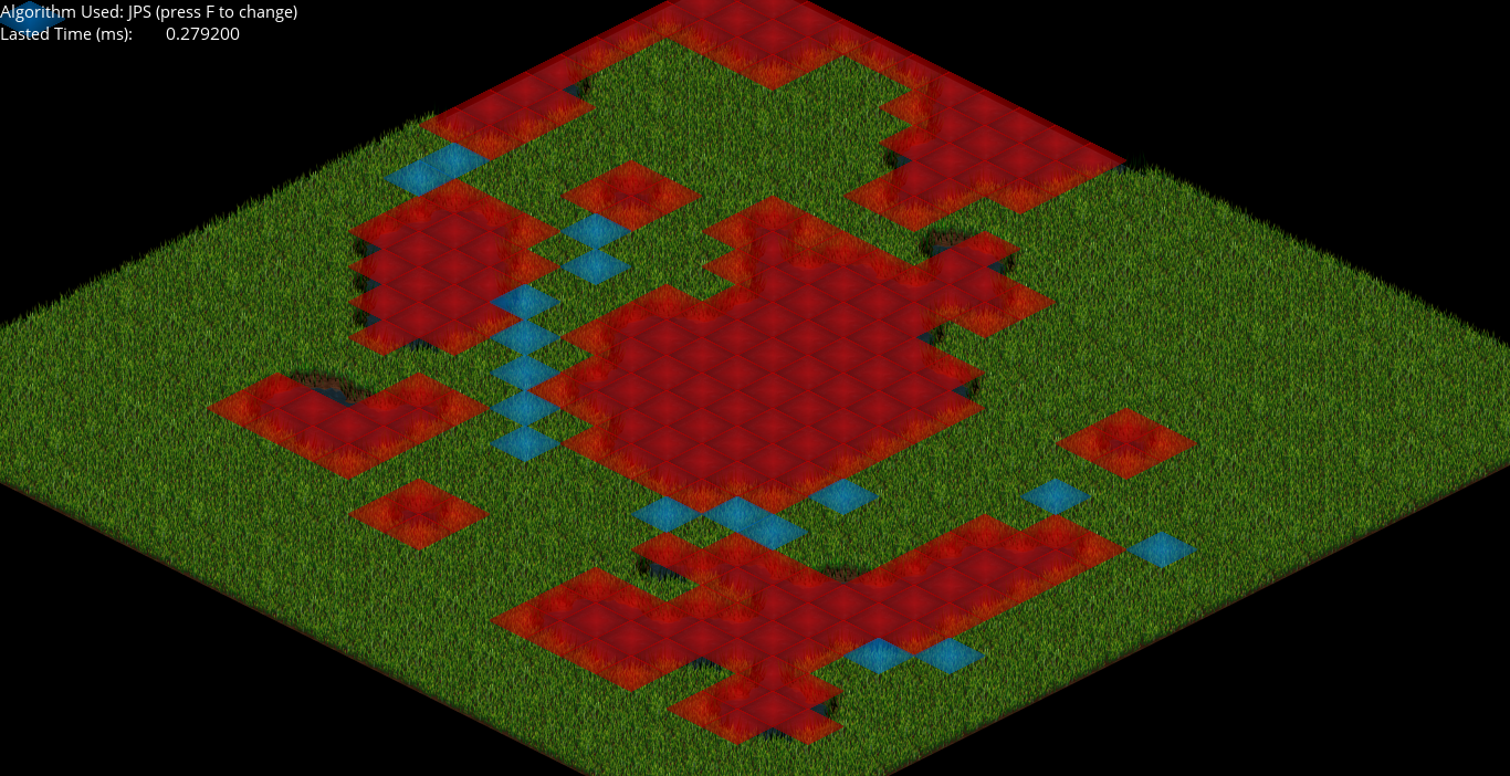
Now, with Jump Point Search implemented we can take measures! In the exercise, the Scene Module is ready to pick pathfinding measures (which are shown both in output and screen). If we run both algorithms for the same path, we can check how many steps (this only in the console output area in Visual Studio) each one did (or how many nodes exploring) and how fast they come up with a path for the same start/end points. So first I tested it in a map done with Tiled of 25x25. In Debug mode the results were this (note that, in all the images, the blue tile that is outside the map and not in the path is a tile that marks the mouse position to select start/end nodes when calling a path, but mouse is not seeable in screen captures):

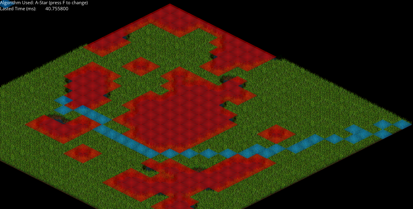
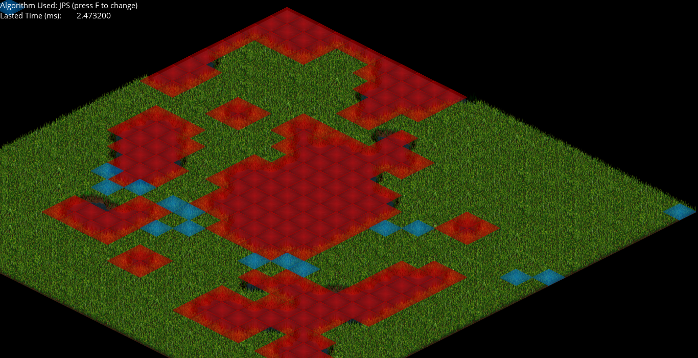
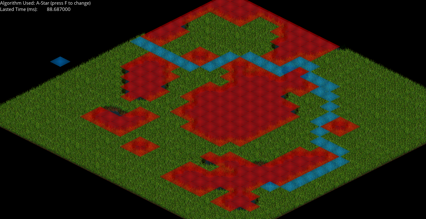
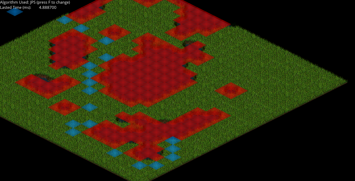
If the images are not properly seen, click on them to open up and see them bigger (you will see correctly the time that each algorithm, for the same path, lasts). Then I tried it in Release mode to see how it was in run-time:

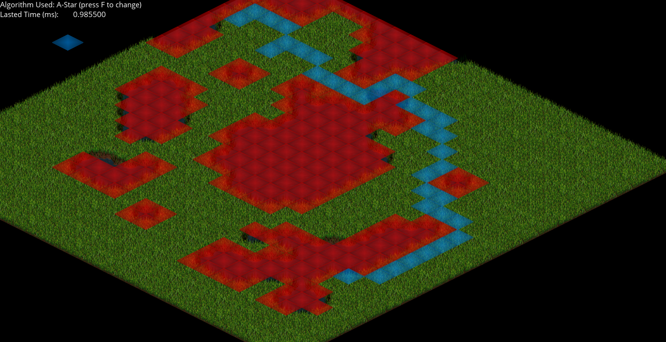
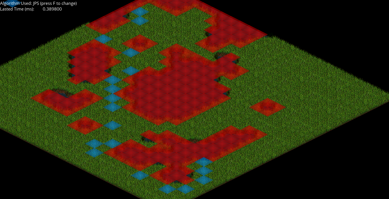
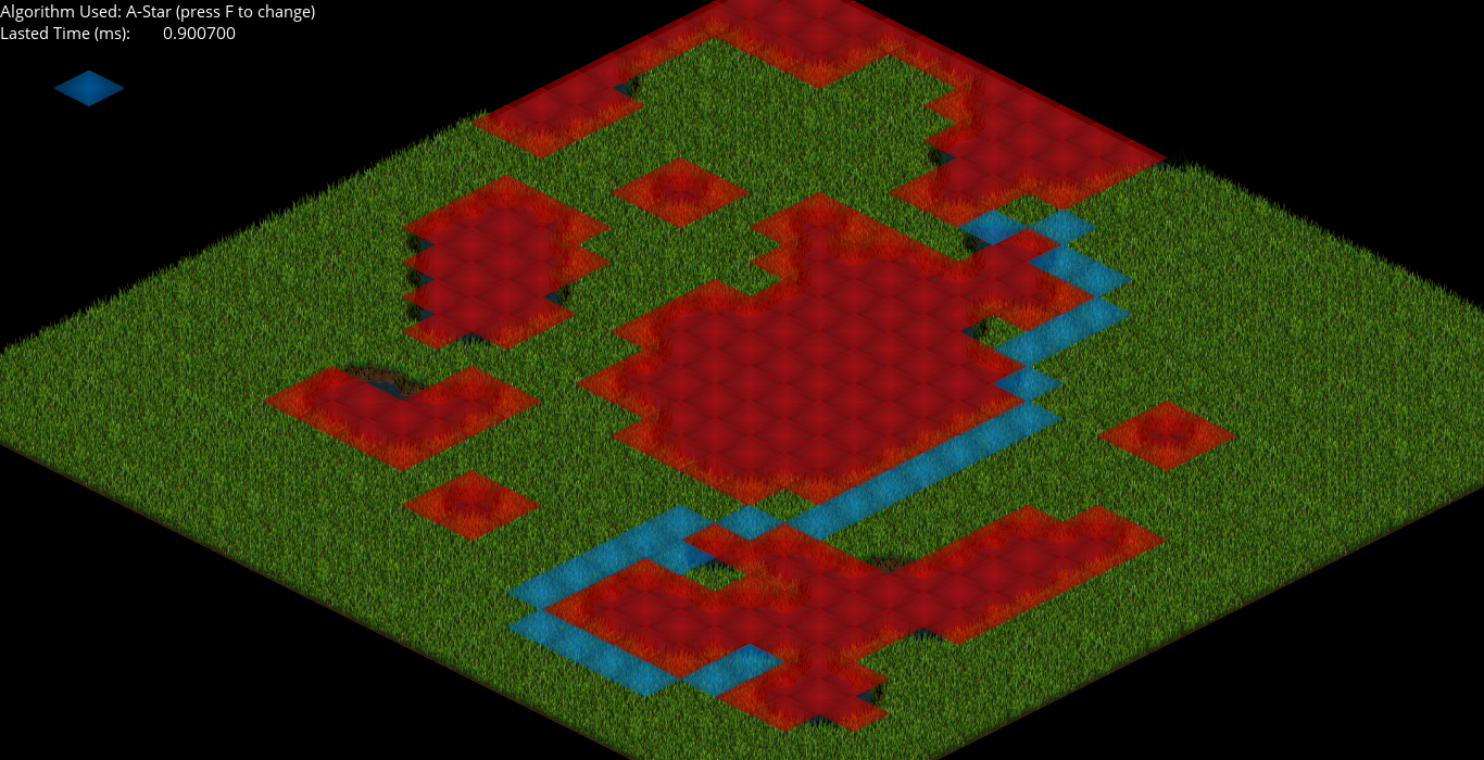
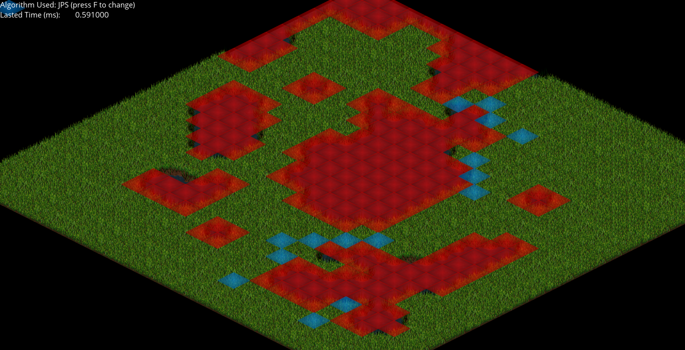
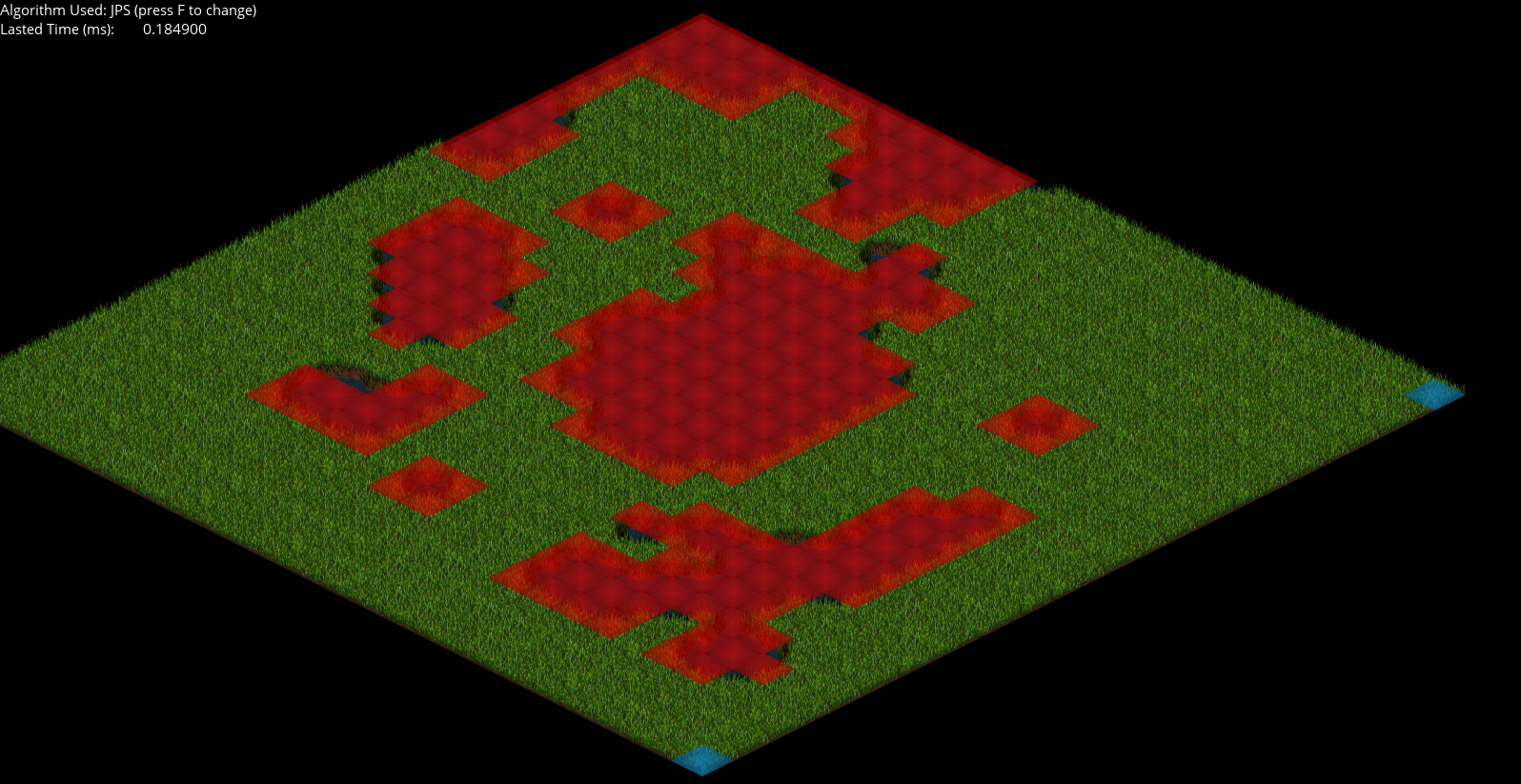
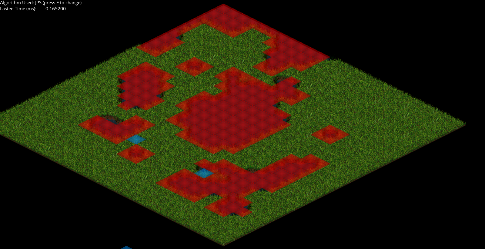
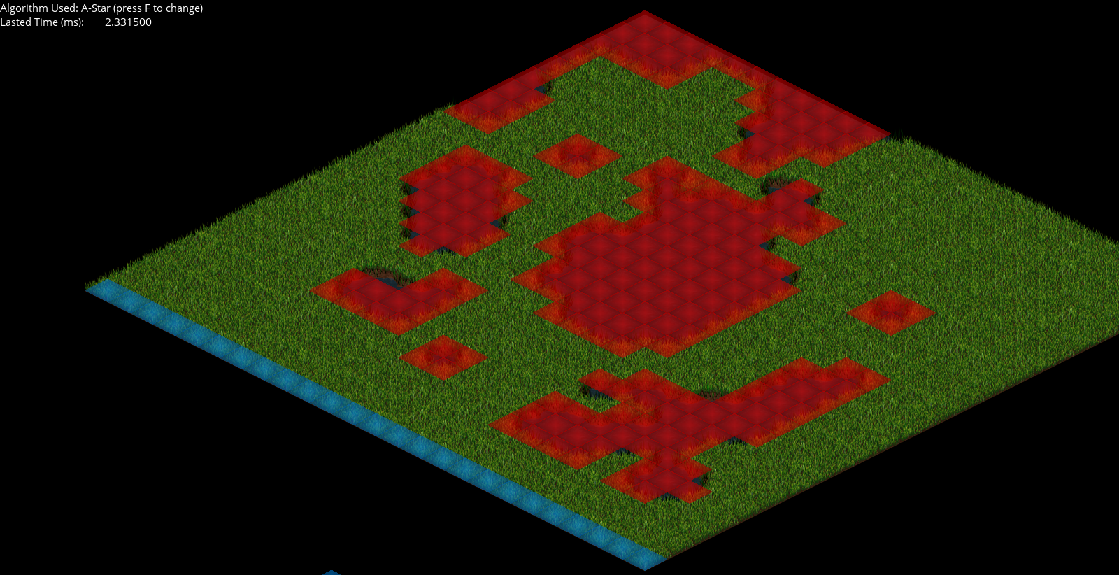
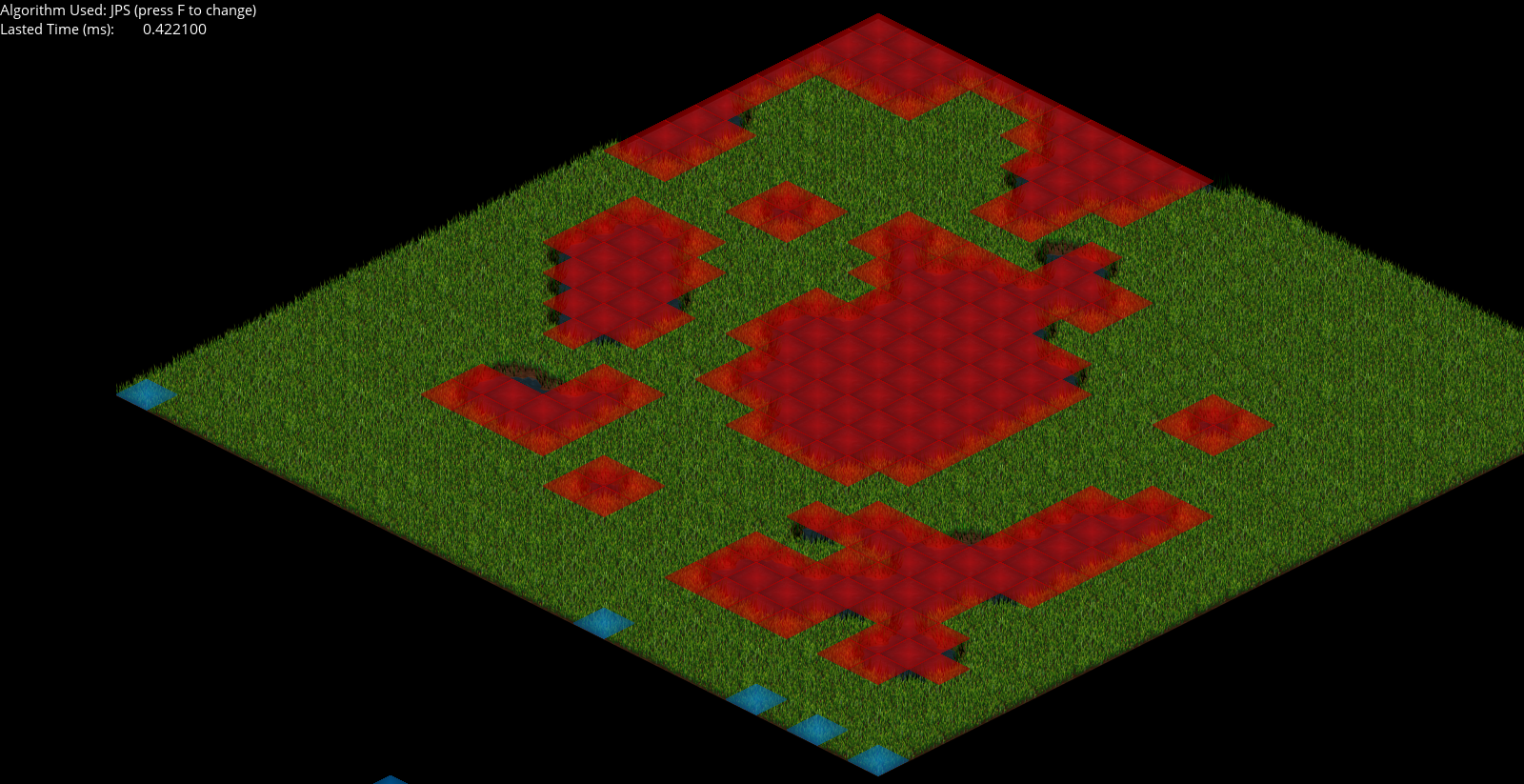
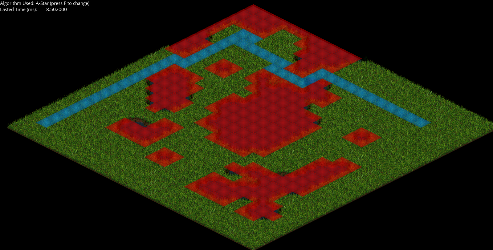
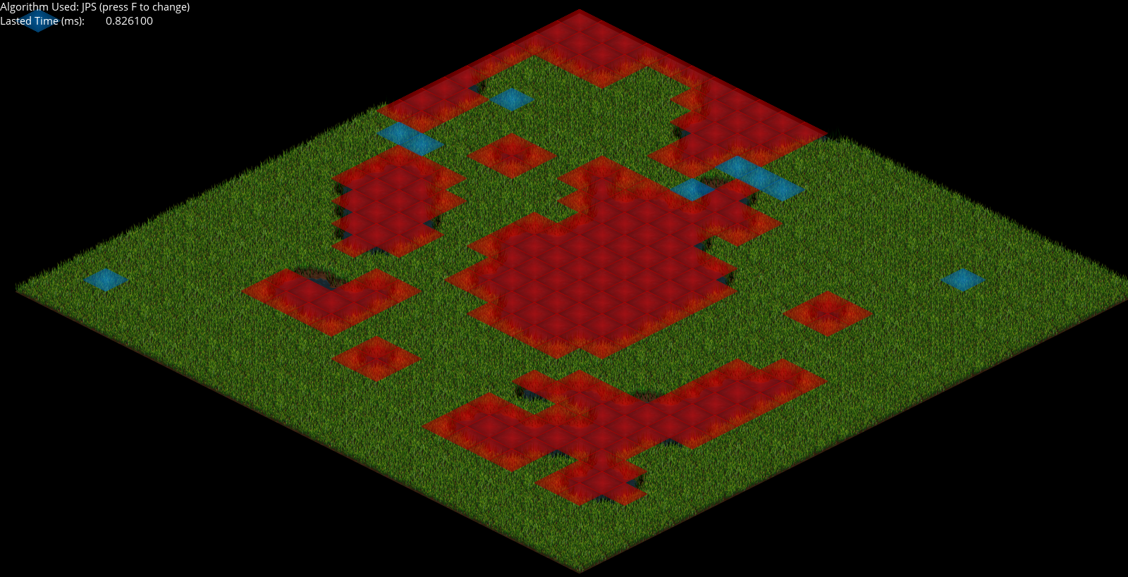
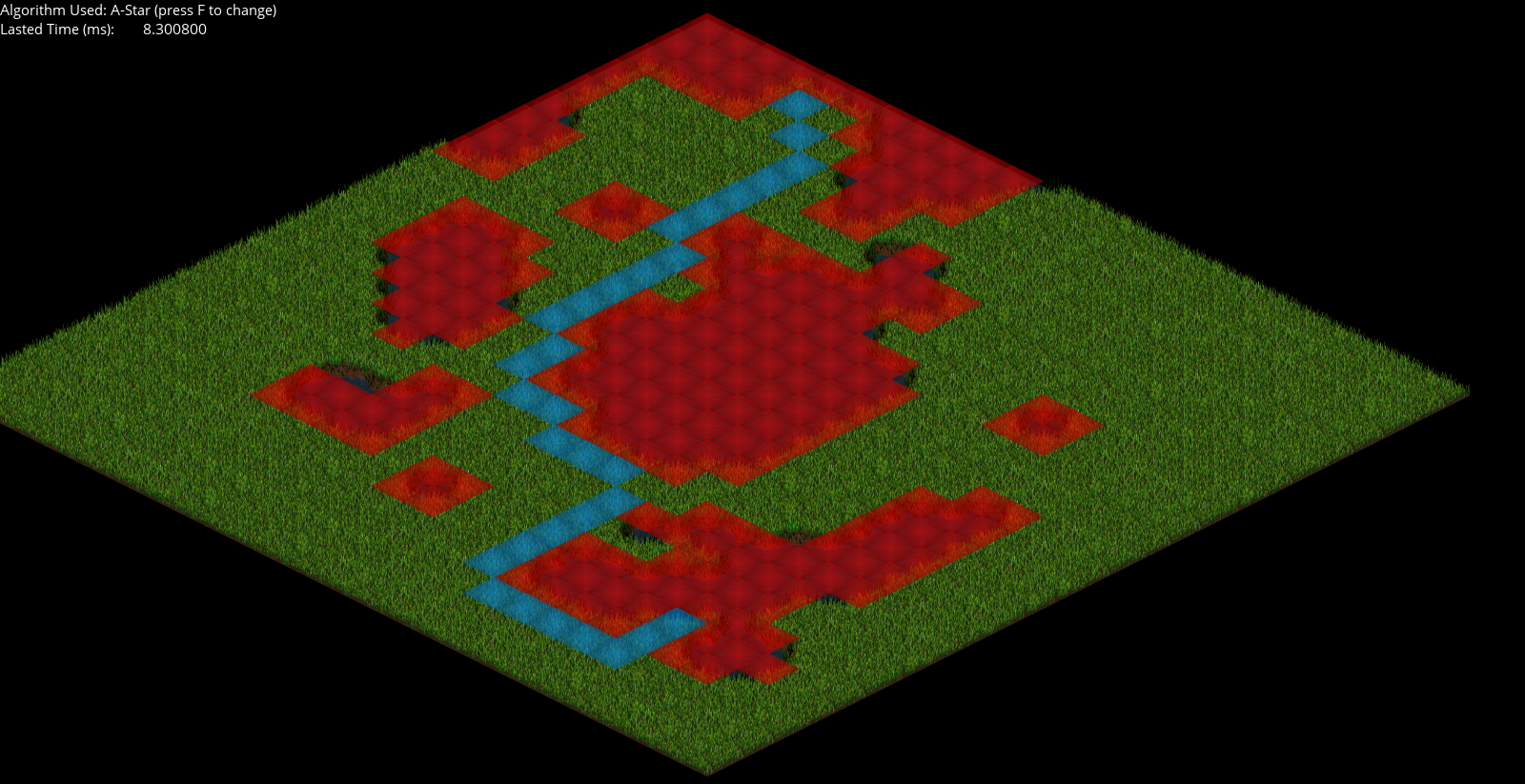
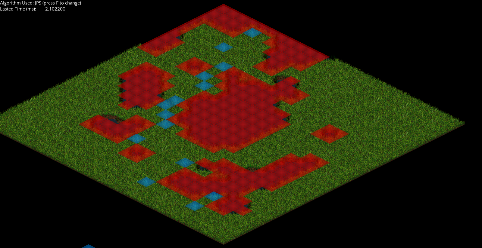
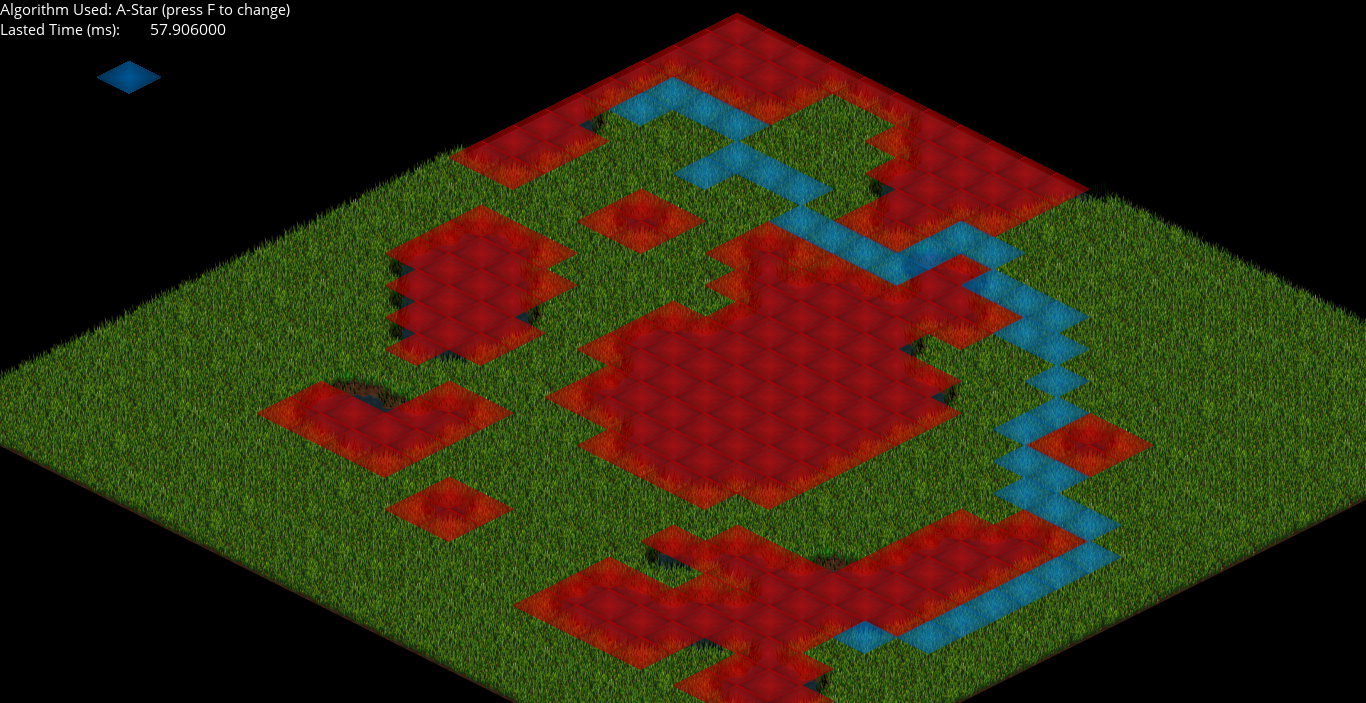
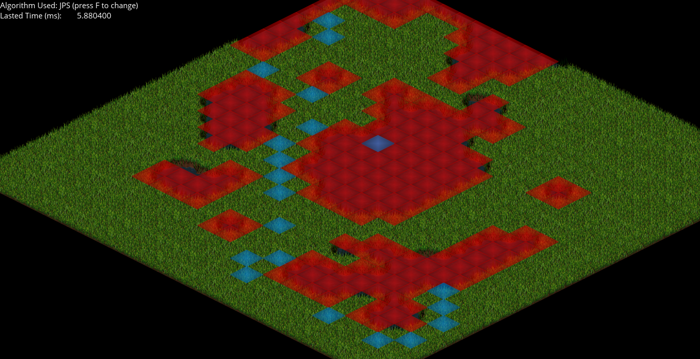
Here I was a bit surprised because in Release mode the difference is not that much, so I felt like the effort of all this (of the algorithm that supposed to improve A* a lot) was useless. But then I come up with a little detail: this was a map of 25x25. Big games like Company of heroes, as mentioned above, use very huge maps in their games, as Chris Jurney said (this is explained in the section of Other Games’ Approach, concretely in the part of Company of Heroes and Dawn of War 2), maps up to 250 000 cells. So I thought on make A* fight JPS in a map of the dimensions of one of the maps in the project I’m currently doing in university for Project II subject, which have, approximately, 100 000 tiles (350x350). I even cut that map because in the system used for this research (the same for the exercise in the upper section) I didn’t had a way to optimize map rendering and was very slow (to the point that I couldn’t test it properly), so I did a very improvised map of 150x150 (in which I still have a bit slow map rendering but it was okay for testing this) and run it on Release (since the huge improvement in Debug mode was already proven), and the optimization is incredible (note that green grass parts are acting as colliders, this is because I did the map very fast with the thing I had in there in hand, but it serves to our testing purposes):

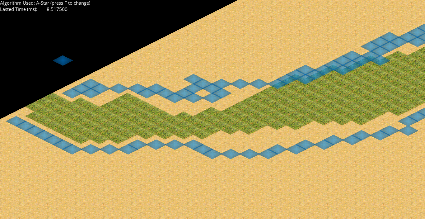
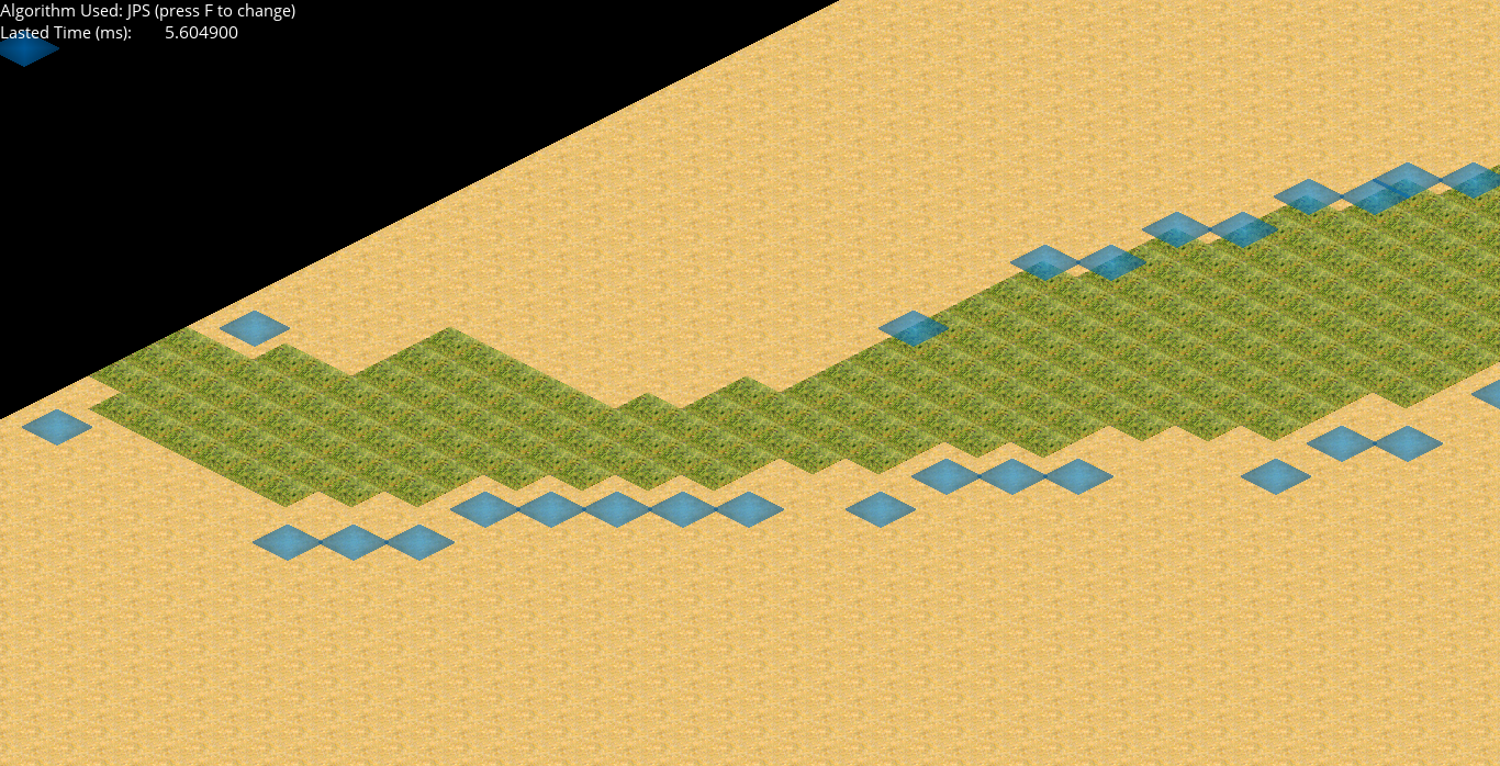
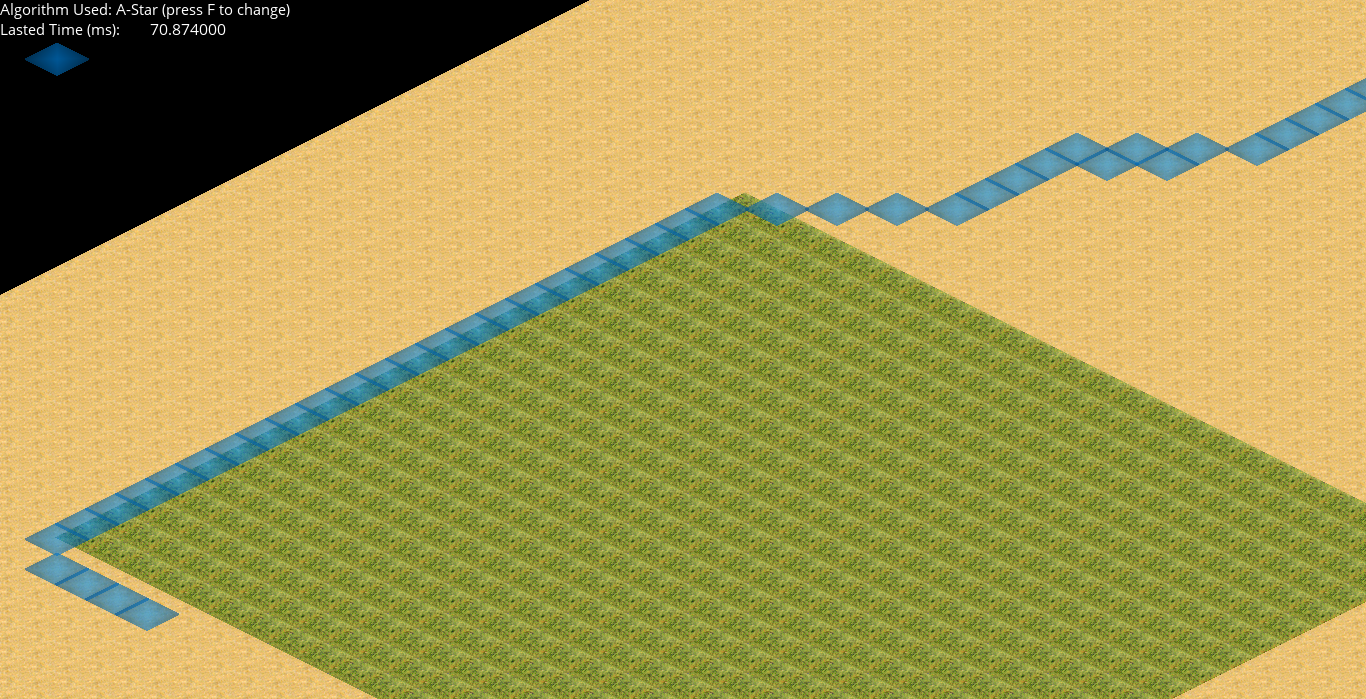
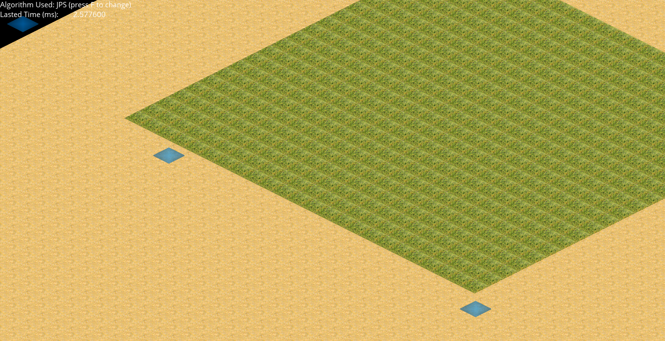
As you can see, in the second test, JPS skips lots of nodes and is way faster. I just see it running 35 times faster than A*, but the map is 150x150, maybe in a bigger map with bigger paths calculations and more (and cleverly designed) obstacles, can reach a way higher optimization.

If you want to see it with your eyes, go to the upper C/C++ Implementation section and download the code. You can do the exercise or see it in the solution. You can try it in both maps just by changing the path used to call the map to load in line 36 of j1Scene.cpp. Is an if() statement, you can use the one called “iso_walk.tmx” (the little map of 25x25) or the one called “iso.tmx” (the big desert map). By default, the little one is called, but just comment the if() statement that I told and uncomment the other one and will change the map (be careful because in the big map, A* might crash, I suspect that is because it cannot hold that big paths, but I’m not sure).

Other External Results

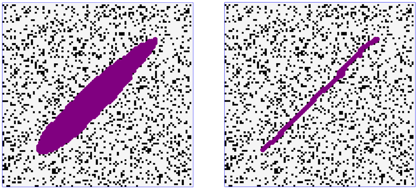
If, you are not implementing JPS with the system I provide (or you can’t see the measures or want to see other external results to prove JPS efficiency), you can check the next pictures provided by Daniel Harabor of its own results in different maps:

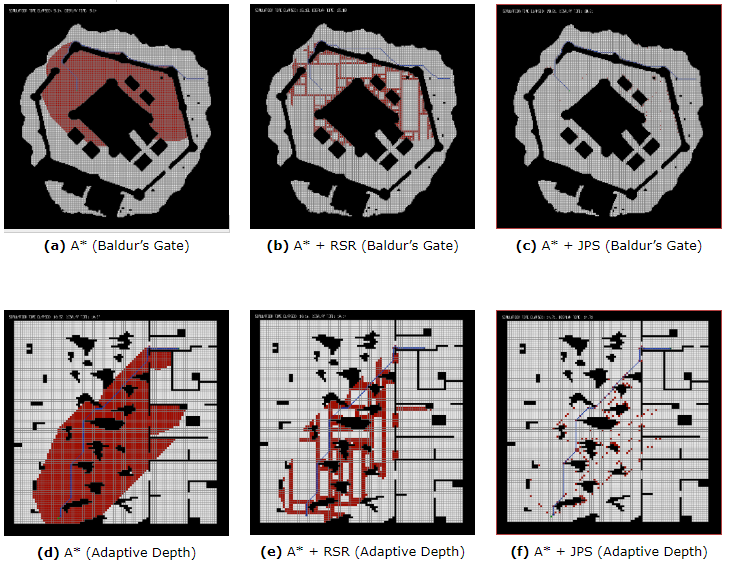
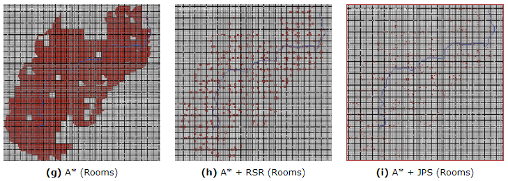
They show how many tiles are explored by A, A with the RSR optimization (explained below) and A* with JPS optimization. Harabor also compared to two other algorithms (Swamps and HPA*, talked about it above). This results are presented in the paper in which Harabor presented JPS.

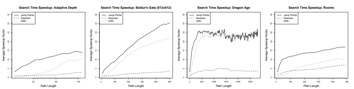
As you may see, sometimes HPA* can be as performatic as JPS. For that reason (and because it has other advantages), downwards, we will talk a bit about HAA*, an HPA* variant. Also, you can checkout this visual and interactive page to see how many pathfinding algorithms work and how much they last to come up with a path (including JPS, be careful because if you choose, in JPS, to show recursion, will visually last because will show the full recursion, but the real lasted time is shown in the bottom left corner). Finally, here there is a video in which JPS is run several times in a big maze showing how much time lasts on finding a path (at the bottom right corner), and, in this video, they compare JPS and A* performance on the same maze with the same paths (watchout! In there is like a thousand times faster!).

More Information on JPS and Sources

With the results that Jump Point Search give, we can see that is a heavy improvement for A* algorithm. If you still don’t understand it, you can check this page that gives a more visual explanation of JPS (and you can even try the algorithm!). Also, Daniel Harabor has a page in his blog (the same than Rectangular Symmetry Reduction and Path Symmetries) explaining it in a more informal and understandable (less mathematical) way than in the paper linked downwards.

There is another explanation with code and visual examples and a video with a step by step JPS.

If you have understood it and still have some curiosity, you can read this paper in which many Artificial Intelligence experts (including Harabor) make compete many algorithms in some different maps and see another video showing different pathfinding ways.

And finally, you can see the paper in which Harabor and Grastien presented JPS (and a summary).

All the links in this section (except some of the videos) were the basis to building it.

Jump Point Search Improvements

There are some improvements that can speed up even more JPS and which you can explore. Harabor and Grastien present some improvings such as applying pruning rules over many nodes at a single time, detecting dead ends and forced neighbours or avoid the jumping over the goal position as well as preprocessing some jump points to make it faster (which actually mades harder to control the changes in the map during the program if any). These changes are presented in this article and you can see a video of a Harabor’s presentation explaining it.

Also there is a talk in GDC Vault at GDC 2015 hosted by Steve Rabin (an specialist in videgames Artificial Intelligence) in which he explains how to pre-compute somethings to speed up JPS and then how to speed up even more by deleting directions towards which to explore by implementing a technique taht he calls “Bounding Goal”, which is kind of making a bounding box around optimal nodes that we can reach and decide the directions towards which to explore.

---

*Many information? Looking for other section? Go back to Index

Other Improvements

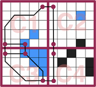
Rectangular Symmetry Reduction (RSR)

Rectangular Symmetry Reduction is an algorithm that checks and eliminates path symmetries by decomposing a map into empty rectangles (meaning that they have no obstacles inside) pathfind by only expanding nodes in the perimeter of those rectangles (not in the inside). RSR is very effective and fast for maps with large open areas or which can be naturally decomposed into rectangular regions. It follows the next steps:

1. Decompose the grid into empty rectangles (size of rectangles can vary according to map size and obstacles on it) and prune the nodes inside of them.
2. Connect nodes of the perimeters of a rectangle with nodes in other perimeters.
3. When a origin/destination is located inside a rectangle, a temporarily procedure is performed by connecting these nodes to the nearest 4 perimeter nodes.

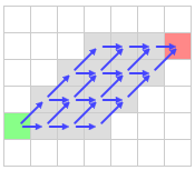
At the end, RSR looks like this (arrows are the macro edges):

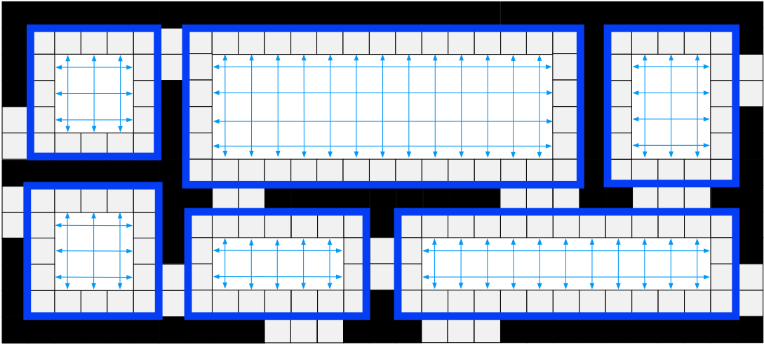
RSR is pretty simple to understand, quick to apply, preserves optimally and has low memory overheads. If we combine it with another search algorithm, it can speed it up considerably.

Regarding memory, the only things to store are the IDs of the parent rectangle of each traversable node in the map and the dimensions and origin of each rectangle, so in the worst case we need until 5n integers.

Check out this blog page of Daniel Harabor (the developer of RSR), which explains it visually and understandably. He also leaves there access to its papers to check RSR deeply.

Hierarchical Annotated A* (HAA*)

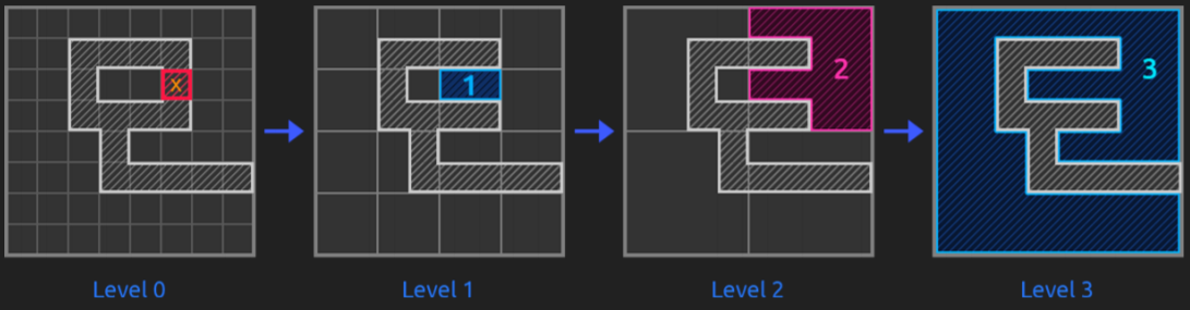
Hierarchical Annotated A* (HAA* ) extends HPA* by dividing a map into traversable terrain and blocked areas (as traditional) but doing a detailed analysis on the different terrains that the traversable parts might have (and the costs), like water, sand… This makes that the units that must move over the map have into account the terrain which they are passing through (since the path does it), allowing to have a map with different terrain types with an optimized pathfinding that can be efficiently supported in a game like an RTS. Also, it allows the moving of units with variable sizes. This approach is interesting because very little works focused on diverse-size moving elements and different terrain types (with different costs), case in which JPS or RSR might not be a good idea for you.

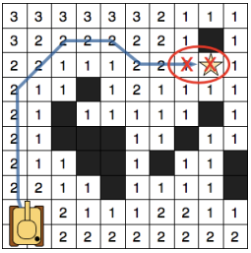
The basis for HAA* is to have a clearance value (a distance to obstacle) which is thought as the amount of traversable space and is used to do a fast guess if a moving element of a determined size will be able to cross a map area (this idea, explains Harabor, was extracted from an algorithm called Brushfire, for robotics). It first assign a value of 1 to each tile aside a static obstacle. Then, their immediate neighbours are assigned with a 2, then, their neighbours with a 3, and keeps going until it all tiles have a value. With this, we can compare the moving elements with the capability of passing through or not.

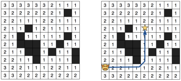
For big units, a path can look like this (notice that there are many tiles in black because it only considers values bigger than 1, it does not mean that they are non-traversable):

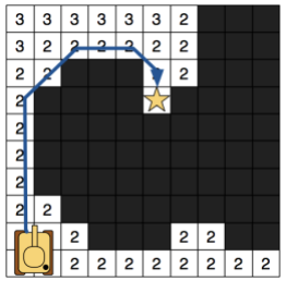
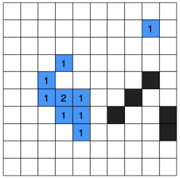
But this can give path problems like this, in which the tank should be able to pass but the path calculates that it doesn’t:

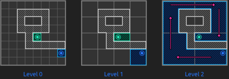
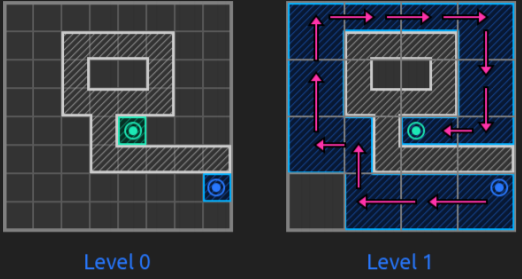
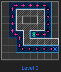
This is solved by Harabor (linked downwards), by doing what he calls “true clearance”, which is, instead of considering each tile individually to assign a clearance value, it considers groups of tiles. It’s done by surrounding each tile with a 1x1 square and, if the tile is traversable, a clearance value of 1 is assigned. Then this square is expanded symmetrically down to the right incrementing clearance value, and does so until it detects an obstacle or limit within that square. It looks like:

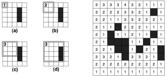
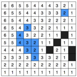
Being a, b and c the square expansion, d the moment in which stops and the right image the final result, with which the problem seen before would be solved. Now the question is how to process different terrain types. Well, the solution is simple, we first assign clearance values to all the map without considering the terrain type, just as we did before (only considering if an area is or is not walkable). Then, we assign clearance values for each terrain type considering other terrains also as non-traversable. Finally, we sum the both layers of clearance values. The process for sand (white) + water (blue) and result are:

This uses more memory than other methods, but allows to have a pathfinding that has into account moving units sizes and terrain types.

So, the algorithm has two parts, a modification of A* and a Hierarchical part. This modification of A* (called Annotated A* ) consists on passing to the function (a part of its usual parameters), the size and the capability of the moving element and then, when exploring a node, it checks if its traversable for the size and capability that the element has, being a tile traversable if the clearance value is (at minimum) equal to the agent size and the terrain traversable according to the capability. Everything else, is the same than A*.

On top of this algorithm, a hierarchical abstraction is made to speed up. To have it is difficult since, with different terrain types, it must be as approximate as possible that can be as representative of the map as possible. To achieve that, first the map is divided into adjacent Clusters connected with entrances (consisting on two tiles of the both connected clusters that must be of the same terrain type), allowing to represent terrains accurately in this hierarchical representation (event though seems to contain redundant or duplicated information).

Here you will find an article of AI Game Dev written by Daniel Harabor about HAA* (used for this section) in which it links to this bigger paper explaining it better. In that article, they also purpose optimizations for this system which decrease the memory used and increase performance by optimizing both the map representation and the algorithm. Also, it shows an analysis on performance, proving that is a fast and good approach to tackle games that feature different terrain types and mobile unit sizes.

---

*Many information? Looking for other section? Go back to Index

Final Thoughts and Recommendations

After all the information gathered here, I think that a conclusion is needed. There are lots of manners to improve A* ‘s pathfinding, to make it faster, to make it lighter… So we have to take a balance and put in there many things to have into account. First of all, we have to know what our game needs in terms of pathfinding efficiency and memory usage. Maybe, just by improving a bit A* our game runs okay, or maybe we have such a big map and we need a very fast pathfinding… Is a matter of putting into a balance the concepts of optimal and best paths, fastness and memory use as well as how much it cares for our game a realistic pathfinding and things like that.

In more specific terms, talking about Jump Point Search, we have seen that it’s a great A* improvement, but it can happen that is not the best take for our game, for that reason I introduce you Rectangular Symmetry Reduction and Hierarchically Annotated A*, the three of them developed by Daniel Harabor, for the cases in which JPS is not helpful. This can be the case if your map has different terrains with different crossing weights (case in which you will need to give memory and speed) or if you want precise and realistic paths (same case, less speed and memory but more good-looking IA). For this reason, and because he is the creator, I have been emailing Daniel Harabor with questions regarding this matters, and, rather than being me the one that gives you some recommendations on what pathfinding to use and when and which guidelines to follow, let him be the one telling you.

I will transcribe here my questions and annotations on bold letters and his answers are the ones in the squares. In a case we mention SRC, a short path algorithm that spends more memory to increase speed (decreasing pathfinding time until the order of nanoseconds). It was the fastest algorithm in a competition of grid path planning of 2014. In the link, there is an overview, but I didn’t inquired much on it because at that moment I was just looking over SRC and it seemed very complex to implement (and was not the main focus for my purposes because of the memory that needs).

With no more delay, here is the conversation:

Hi Lucho, 

Thank you for the email; it’s always nice to hear from a fellow
pathfinding enthusiast! I am happy to read that you found my
research interesting and I am humbled by your kind assessment
of it. I will try my best to answer your questions below, inlined

The first question is related to JPS against SRC. I have seen that SRC is way faster than JPS but spends lots of memory, so would you recommend better to use JPS instead of SRC? (you know, since I feel that the improvement in the speed it’s not worth with that memory usage in a context like an RTS videogame).

A main advantage of JPS is that it runs online. That means if the
map changes (e.g. your workers clear a new path through the forest,
or your sappers blow up a bridge) then any subsequent shortest path
searches will take those changes into account. SRC meanwhile assumes
the map will remain static. Paths are computed faster than JPS and
it’s also possible to extract just the first few steps of a path instead
of searching all the way to the target. This can be advantageous because
replanning is fast. The main price, as you know, is the offline preprocessing
overhead of SRC and the online memory overhead.

Which method is better depends on the situation. In games such as Dragon Age
for example, the maps are not so big (usually < 100K tiles) and the space and
time overheads are usually small.

In the last period I have been thinking about combining the advantages of JPS
and SRC. There are a few ways to do this. One way is to combine the SRC
database with a jump point database. In such a setup the SRC database tells
the user which direction to take to reach the target and the jump point database
tells how many steps to take in that direction before the path needs to turn.
The preprocessing costs are the same as SRC and the memory overhead is similar.

You can read more here:

http://harabor.net/data/papers/sbghs-toppgm-18.pdf

Then I was thinking on rectangular symmetry reduction. Do you think it’s a good idea to mix it with JPS? I don’t even know if that is possible.

RSR has two advantages vs JPS:
 1. Rooms are precomputed so there’s no grid scanning*
 2. Rooms limit the area in which neighbours are found (JPS scans are only
 limited, in the worst case, by hitting the edge of the map).

It’s possible to add both of these advantages to JPS by: 

 (a) precomputing jump points and,
 (b) limiting the maximum distance for any jump to some fixed value k.

You can find out more here:

http://harabor.net/data/papers/harabor-grastien-icaps14.pdf
https://www.youtube.com/watch?v=NmM4pv8uQwI

And finally, for videogames in which the nodes of the graph are weighted because of different terrains, I imagine that JPS might not be a very good idea, so what would you recommend to use? I was guessing that RSR or HAA*, but I might be wrong, so I wanted to confirm it.

This is a great question. In dynamic cost settings JPS will no longer
guarantee to return the optimal path. The interesting point here is that
symmetries still exist and they might also be fruitfully exploited. RSR
could be used for this purpose but I have never tried that experiment.
HAA* and SRC will also work in this setting.

If your map is also dynamic, you might consider e.g. weighted A* (which is
bounded suboptimal) or some type of anytime search (which returns a best
path it can find for a given time limit).

And here ends the conversation. I think that with this, we can already have an idea of which pathfinding areas to explore according to our game, but remember, we must avoid things like this:

(If you can’t see the video, see it here).

Links to Additional Information

All the information that I have used to build this research is linked all over the text in their respective sections or directly given. Also, you can find more interesting links and additional information (from which I also extracted information) here:

• Discussion on different pathfinding algorithms, explanations and links to articles explaining them.

• Full A* guide in Amit’s Thoughts on Pathfinding page at Red Blob Games.

• The thesis of Daniel Harabor on pathfinding and its blog pages about pathfinding via symmetry breaking, which are together in this document

• Survey Document on recent work in pathfinding in games by Adi Botea, Bruno Bouzy, Michael Buro, Christian Bauckhage and Dana Nau.

• AI Game Dev page from where I extracted many articles and GDC Talks from which I extracted many information (linked them in their corresponding section of this page). Many of the ones I used (bot of AI Game Dev and GDC Talks) I compiled their links on this pdf (be careful because AI Game Dev page is no longer available, to see their articles, you will have to search the AI Game Dev page in Internet Web Archive).

You can also find curious information on looking for other kind of approaches to perform pathfinding (of course, for understandable reasons, I didn’t put here all the existing ways) or other curious investigations such as LEARCH, a combination of machine-learning algorithms used to teach robots how to find near-optimal paths on their own, based on neural networks. This paper mentions some about it, can be interesting (I didn’t read it deeply).

Thanks

I can’t leave without thanking people and entities that provide some help when building all this, either with a small e-mail, a big answering e-mail or just by supporting the research. Thanks Yatch Games, Beautifun Games, Rick Pillosu, Marc Garrigó, Roger Leon and especially to Daniel Harabor. And, finally, thanks to you, reader. If any trouble with anything I explain, you can find me on my GitHub or e-mail me to luchosuaya99@gmail.com

---

*Many information? Looking for other section? Go back to Index